Tutorials
Every tutorial below is a runnable script in the repository’s examples/
directory: parameters at the top, no main(), only the public API, and each
is smoke-tested in CI (tests/test_examples.py) so the code on this
page always runs. Copy a script, edit the parameter block, and go.
Run any of them directly:
python examples/fixed_boundary_run.py
The light scripts finish in a few seconds once JAX has compiled; the free-boundary and optimization scripts are heavier (see each section).
Getting started
Fixed-boundary run
Read an &INDATA deck, converge the equilibrium on the multigrid ladder with
VMEC2000-format progress printing, and write and plot the wout. This is the
three-step workflow every new user needs.
#!/usr/bin/env python
"""Fixed-boundary VMEC run: input file -> solve -> wout -> plots -> Boozer.

The three steps every new user needs: read an ``&INDATA`` file, converge the
equilibrium on the NS_ARRAY multigrid ladder (VMEC2000-style progress
printing), and write/plot the results.  CLI equivalent of this script:
``vmec examples/data/input.li383_low_res --booz``.

Physics: the LI383 (NCSX-class, nfp=3) stellarator boundary at low
resolution, zero pressure.  Expected runtime: ~1 min on a laptop CPU on the
first run (XLA compilation, cached persistently), a few seconds afterwards.
Achieved: converges to FTOL = 1e-13; the wout scalars printed at the end
(aspect ~ 4.4, volume ~ 2.96 m^3) match VMEC2000 to Appendix-A tolerances.
"""

import dataclasses
import os
from pathlib import Path

import vmex as vj

# --------------------------- parameters ------------------------------------
INPUT_FILE = Path(__file__).resolve().parent / "data" / "input.li383_low_res"
OUT_DIR = Path("output_fixed_boundary_run")
RUN_BOOZER = True          # Boozer spectrum via booz_xform_jax (optional dep)
CI = os.environ.get("VMEX_EXAMPLES_CI") == "1"  # smoke-test mode

# --------------------------- read the input --------------------------------
inp = vj.VmecInput.from_file(INPUT_FILE)
if CI:  # reduced budget for the CI smoke test
    inp = dataclasses.replace(inp, ns_array=[13], ftol_array=[1e-8],
                              niter_array=[2000])
print(f"input: {INPUT_FILE.name}")
print(f"  nfp={inp.nfp}  mpol={inp.mpol}  ntor={inp.ntor}  lasym={inp.lasym}")
print(f"  ns_array={list(map(int, inp.ns_array))}  "
      f"ftol_array={[f'{f:.0e}' for f in inp.ftol_array]}")
print(f"  major radius RBC(0,0) = {inp.rbc[inp.ntor, 0]:.3f} m, "
      f"phiedge = {inp.phiedge:.3f} Wb")

# --------------------------- solve ------------------------------------------
result = vj.solve_multigrid(inp, verbose=True)  # prints VMEC2000-format tables
print(f"\nconverged = {result.converged} after {int(result.iterations)} "
      f"iterations; fsqr = {float(result.fsqr):.3e}, "
      f"fsqz = {float(result.fsqz):.3e}, fsql = {float(result.fsql):.3e}")

# --------------------------- write the wout file ----------------------------
wout = vj.wout_from_state(
    inp=inp, state=result.state,
    fsqr=float(result.fsqr), fsqz=float(result.fsqz), fsql=float(result.fsql),
    niter=int(result.iterations), converged=bool(result.converged),
)
OUT_DIR.mkdir(parents=True, exist_ok=True)
wout_path = vj.write_wout(OUT_DIR / "wout_li383_low_res.nc", wout)
print(f"\nwout scalars: aspect = {float(wout.aspect):.4f}, "
      f"volume = {float(wout.volume_p):.4f} m^3, "
      f"B0 = {float(wout.b0):.4f} T, betatotal = {float(wout.betatotal):.3e}")
print(f"wrote {wout_path}")

# --------------------------- plots ------------------------------------------
figures = vj.plot_wout(wout_path, OUT_DIR)  # summary/surfaces/modB/profiles/3d
for key, path in figures.items():
    print(f"wrote {path}")

# --------------------------- Boozer spectrum (optional) ---------------------
if RUN_BOOZER and not CI:
    try:
        boozmn_path = vj.run_booz_xform(wout_path, outdir=OUT_DIR)
        for key, path in vj.plot_boozmn(boozmn_path, OUT_DIR).items():
            print(f"wrote {path}")
    except ImportError as exc:
        print(f"skipping Boozer step ({exc}); pip install booz_xform_jax")
All diagnostics and the Boozer transform
vmex ships its plotting and its Boozer transform in the box. This produces
every plot_wout figure (flux-surface summary, cross-sections, |B|,
profiles, 3D render) and the straight-field-line Boozer |B| spectrum on the last closed
flux surface — the view used to judge quasisymmetry.
#!/usr/bin/env python
"""All the built-in diagnostics: solve -> every ``plot_wout`` figure -> Boozer.

vmex ships its plotting and its Boozer transform in the box, so a single
converged equilibrium gives you the whole diagnostic set with no external
tooling.  This script walks the two calls that matter:

- ``vj.plot_wout`` writes the five standard figures (flux-surface summary,
  nested cross-sections, |B| on a surface, the radial profiles, and a 3D
  render) and returns ``{key: path}``;
- ``vj.run_booz_xform`` + ``vj.plot_boozmn`` transform to straight-field-line
  Boozer coordinates and plot the |B| spectrum on the LCFS -- the view used to
  judge quasisymmetry.

CLI equivalent: ``vmec examples/data/input.li383_low_res --plot --booz``.

Physics: LI383 (NCSX-class, nfp=3), zero pressure.  Expected runtime a few
seconds warm; the Boozer step needs the optional ``booz_xform_jax`` package and
is skipped with a message if it is absent.
"""

import dataclasses
import os
from pathlib import Path

import vmex as vj

# --------------------------- parameters ------------------------------------
INPUT_FILE = Path(__file__).resolve().parent / "data" / "input.li383_low_res"
OUT_DIR = Path("output_plot_and_boozer")
WHICH = ("summary", "surfaces", "modB", "profiles", "3d")  # all plot_wout kinds
RUN_BOOZER = True                                          # optional dep
CI = os.environ.get("VMEX_EXAMPLES_CI") == "1"         # smoke-test mode

# --------------------------- solve a small equilibrium ---------------------
inp = vj.VmecInput.from_file(INPUT_FILE)
if CI:  # single coarse grid keeps the smoke test to a few seconds
    inp = dataclasses.replace(inp, ns_array=[13], ftol_array=[1e-8],
                              niter_array=[2000])
result = vj.solve_multigrid(inp, verbose=not CI)
wout = vj.wout_from_state(
    inp=inp, state=result.state,
    fsqr=float(result.fsqr), fsqz=float(result.fsqz), fsql=float(result.fsql),
    niter=int(result.iterations), converged=bool(result.converged),
)
OUT_DIR.mkdir(parents=True, exist_ok=True)
wout_path = vj.write_wout(OUT_DIR / "wout_li383_low_res.nc", wout)
print(f"converged = {result.converged}; wrote {wout_path}")

# --------------------------- every wout figure -----------------------------
# plot_wout accepts a WoutData or a path and returns {key: written_png_path}.
figures = vj.plot_wout(wout_path, OUT_DIR, which=WHICH)
for key, path in figures.items():
    print(f"  [{key:9s}] {path}")

# --------------------------- Boozer spectrum on the LCFS -------------------
# booz_xform_jax is optional; guard the import so the core workflow always runs.
if RUN_BOOZER:
    try:
        boozmn_path = vj.run_booz_xform(wout_path, outdir=OUT_DIR)
        print(f"wrote {boozmn_path}")
        for key, path in vj.plot_boozmn(boozmn_path, OUT_DIR).items():
            print(f"  [booz:{key:9s}] {path}")
    except ImportError as exc:
        print(f"skipping Boozer step ({exc}); pip install booz_xform_jax")
VMEC++ JSON input
vmex reads both the classic &INDATA namelist and the VMEC++ JSON schema,
and can write the JSON form — a drop-in for either ecosystem. This converts a
deck, reads it back, and confirms the two representations describe one
equilibrium.
#!/usr/bin/env python
"""VMEC++-style JSON input: convert an &INDATA deck, round-trip, solve.

vmex reads *both* the classic Fortran ``&INDATA`` namelist and the JSON
schema used by VMEC++ (``vmecpp.VmecInput``), and can write the JSON form.  So
it is a drop-in for either ecosystem: ``vmec input.json`` and
``vmec input.circular_tokamak`` both work, and this script shows the conversion
and that the two representations describe the same equilibrium.

Steps: read an INDATA deck -> ``inp.to_json`` -> read the JSON back with
``VmecInput.from_file`` (suffix/`{`-autodetected) -> solve -> compare.

Physics: circular tokamak (nfp=1), zero pressure.  Runtime a couple of seconds.
"""

import dataclasses
import os
from pathlib import Path

import vmex as vj

# --------------------------- parameters ------------------------------------
INPUT_FILE = Path(__file__).resolve().parent / "data" / "input.circular_tokamak"
OUT_DIR = Path("output_run_from_json")
CI = os.environ.get("VMEX_EXAMPLES_CI") == "1"


def _solve(inp):
    if CI:
        inp = dataclasses.replace(inp, ns_array=[15], ftol_array=[1e-10],
                                  niter_array=[2000])
    res = vj.solve_multigrid(inp, verbose=False)
    wout = vj.wout_from_state(
        inp=inp, state=res.state, fsqr=float(res.fsqr), fsqz=float(res.fsqz),
        fsql=float(res.fsql), niter=int(res.iterations),
        converged=bool(res.converged))
    return wout


# --------------------------- read INDATA, write JSON -----------------------
OUT_DIR.mkdir(parents=True, exist_ok=True)
inp_indata = vj.VmecInput.from_file(INPUT_FILE)
json_path = inp_indata.to_json(OUT_DIR / "circular_tokamak.json")
print(f"read {INPUT_FILE.name} (&INDATA) -> wrote {json_path} (VMEC++ JSON)")

# --------------------------- read the JSON back ----------------------------
# from_file dispatches on the .json suffix (or a leading '{') to the JSON parser.
inp_json = vj.VmecInput.from_file(json_path)
print(f"read {json_path.name} back: nfp={inp_json.nfp} mpol={inp_json.mpol} "
      f"ntor={inp_json.ntor} lasym={inp_json.lasym}")

# --------------------------- solve both, compare ---------------------------
wout_indata = _solve(inp_indata)
wout_json = _solve(inp_json)
d_aspect = abs(float(wout_indata.aspect) - float(wout_json.aspect))
print(f"aspect: INDATA={float(wout_indata.aspect):.6f}  "
      f"JSON={float(wout_json.aspect):.6f}  |diff|={d_aspect:.2e}")

vj.write_wout(OUT_DIR / "wout_circular_tokamak.nc", wout_json)
print(f"wrote {OUT_DIR / 'wout_circular_tokamak.nc'} from the JSON input "
      "(the two input formats describe one equilibrium)")
Profiles and finite-beta physics
Profile representations
Pressure and rotational transform (or current) can be given as polynomial
coefficients (power_series) or spline knots (cubic_spline). This solves
the same equilibrium both ways and shows they agree, then points to the
NCURR=0 vs NCURR=1 (prescribed iota vs prescribed current) switch.
#!/usr/bin/env python
"""Profile representations: power series vs cubic spline (same physics).

VMEC prescribes the pressure and either the rotational transform (``NCURR=0``)
or the toroidal current (``NCURR=1``) as radial profiles in the normalized flux
``s``.  Each profile can be given as polynomial coefficients (``power_series``)
*or* as spline knots (``cubic_spline`` / ``akima_spline``).  This script solves
the same shaped tokamak twice -- once with power-series profiles, once with the
cubic-spline knots sampled from those very polynomials -- and shows the two
converge to the same equilibrium (aspect, volume, beta agree).  That is the
point: the representation is a modelling convenience, not different physics.

The base deck (``input.shaped_tokamak_pressure``) uses ``NCURR=0`` with a
parabolic pressure ``p(s) = PRES_SCALE * (1 - s)`` and a linear iota
``iota(s) = 1.05 - 0.35 s``.  The commented ``NCURR=1`` block at the bottom
shows the current-prescribed alternative.

Physics: shaped tokamak, finite beta (~few %).  Runtime a few seconds warm.
"""

import dataclasses
import os
from pathlib import Path

import numpy as np

import vmex as vj

# --------------------------- parameters ------------------------------------
INPUT_FILE = Path(__file__).resolve().parent / "data" / "input.shaped_tokamak_pressure"
KNOTS = np.array([0.0, 0.25, 0.50, 0.75, 1.0])       # spline sample locations in s
CI = os.environ.get("VMEX_EXAMPLES_CI") == "1"   # smoke-test mode


def _polyval(coeffs, s):
    """VMEC power-series convention: profile(s) = sum_k coeffs[k] * s**k."""
    return sum(c * s**k for k, c in enumerate(coeffs))


def _terms(coeffs):
    """The meaningful (non-zero-padded) power-series coefficients as floats."""
    arr = np.asarray(coeffs, dtype=float)
    last = int(np.max(np.nonzero(arr))) if np.any(arr) else 0
    return arr[: last + 1].tolist()


def _solve(inp, label):
    if CI:
        inp = dataclasses.replace(inp, ns_array=[13], ftol_array=[1e-10],
                                  niter_array=[3000])
    res = vj.solve_multigrid(inp, verbose=False)
    wout = vj.wout_from_state(
        inp=inp, state=res.state, fsqr=float(res.fsqr), fsqz=float(res.fsqz),
        fsql=float(res.fsql), niter=int(res.iterations),
        converged=bool(res.converged))
    print(f"  {label:14s} converged={bool(res.converged)!s:5s} "
          f"aspect={float(wout.aspect):.4f} volume={float(wout.volume_p):.4f} "
          f"beta={float(wout.betatotal):.4e}")
    return wout


# --------------------------- power-series baseline -------------------------
inp_power = vj.VmecInput.from_file(INPUT_FILE)
print(f"power-series profiles: AM={_terms(inp_power.am)}  AI={_terms(inp_power.ai)}")
wout_power = _solve(inp_power, "power_series")

# --------------------------- equivalent spline knots -----------------------
# Sample the SAME polynomials at the knot locations, then hand VMEC the knots.
am_knots = _polyval(np.asarray(inp_power.am), KNOTS)
ai_knots = _polyval(np.asarray(inp_power.ai), KNOTS)
inp_spline = dataclasses.replace(
    inp_power,
    pmass_type="cubic_spline", am_aux_s=KNOTS.copy(), am_aux_f=am_knots,
    piota_type="cubic_spline", ai_aux_s=KNOTS.copy(), ai_aux_f=ai_knots,
)
print(f"cubic-spline profiles: AM_AUX_F={np.round(am_knots, 4).tolist()}  "
      f"AI_AUX_F={np.round(ai_knots, 4).tolist()}")
wout_spline = _solve(inp_spline, "cubic_spline")

# --------------------------- compare ---------------------------------------
d_aspect = abs(float(wout_power.aspect) - float(wout_spline.aspect))
d_beta = abs(float(wout_power.betatotal) - float(wout_spline.betatotal))
print(f"\nrepresentation-independent: |d aspect| = {d_aspect:.2e}, "
      f"|d beta| = {d_beta:.2e} (the two profile forms describe one equilibrium)")

# --------------------------- NCURR=1 alternative (current-prescribed) -------
# To prescribe the toroidal current instead of iota, set NCURR=1 and give a
# current profile.  The equivalent in-code edit:
#
#   inp_current = dataclasses.replace(
#       inp_power, ncurr=1, pcurr_type="power_series",
#       ac=[1.0, -1.0],          # I'(s) shape; total set by CURTOR
#       curtor=<total toroidal current in A>)
#   wout_current = _solve(inp_current, "ncurr=1")
#
# VMEC then solves for iota self-consistently from the prescribed current.
Finite-beta pressure scan
Ramp the pressure and read three diagnostics straight from the wout: the
volume-averaged beta, the Shafranov shift (outward motion of the magnetic axis),
and the Mercier DMerc interchange-stability profile. Each step is
hot-restarted from the previous equilibrium.
#!/usr/bin/env python
"""Finite-beta pressure ramp: beta, Shafranov shift, and Mercier stability.

Raising the plasma pressure raises beta, pushes the magnetic axis outward (the
Shafranov shift), and eventually threatens interchange (Mercier) stability.
This script ramps the pressure scale of a shaped tokamak, hot-restarting each
step from the previous equilibrium, and reads three diagnostics straight from
the wout:

- ``betatotal`` -- the volume-averaged beta;
- ``raxis_cc[0]`` -- the magnetic-axis major radius; its growth over the
  zero-pressure axis is the Shafranov shift;
- ``DMerc`` -- the Mercier criterion profile (``> 0`` is stable); we report its
  interior minimum.

Physics: shaped tokamak, parabolic pressure ``p(s) = PRES_SCALE * (1 - s)``,
NCURR=0.  Runtime a few seconds (warm-restarted ramp).
"""

import dataclasses
import os
from pathlib import Path

import numpy as np

import vmex as vj

# --------------------------- parameters ------------------------------------
INPUT_FILE = Path(__file__).resolve().parent / "data" / "input.shaped_tokamak_pressure"
PRES_MULTIPLIERS = [0.0, 5.0, 10.0, 15.0, 20.0]   # scales the base PRES_SCALE (-> ~1.5% beta)
NS = 25
CI = os.environ.get("VMEX_EXAMPLES_CI") == "1"
if CI:
    NS = 15
    PRES_MULTIPLIERS = [0.0, 10.0, 20.0]

base = vj.VmecInput.from_file(INPUT_FILE)
base = dataclasses.replace(base, ns_array=[NS], ftol_array=[1e-11], niter_array=[5000])
pres0 = float(base.pres_scale)


def _solve(inp, seed):
    res = vj.solve_multigrid(inp, initial_state=seed, verbose=False)
    wout = vj.wout_from_state(
        inp=inp, state=res.state, fsqr=float(res.fsqr), fsqz=float(res.fsqz),
        fsql=float(res.fsql), niter=int(res.iterations),
        converged=bool(res.converged))
    return res, wout


# --------------------------- pressure ramp ---------------------------------
print(f"{'pres_scale':>11s} {'beta_tot':>10s} {'R_axis(m)':>10s} "
      f"{'Shafranov':>10s} {'min DMerc':>11s}")
print(f"{'-'*11} {'-'*10} {'-'*10} {'-'*10} {'-'*11}")

seed = None
raxis_ref = None
for mult in PRES_MULTIPLIERS:
    inp = dataclasses.replace(base, pres_scale=pres0 * mult)
    res, wout = _solve(inp, seed)
    seed = res.state  # hot restart the next (higher-pressure) point

    beta = float(wout.betatotal)
    raxis = float(np.asarray(wout.raxis_cc)[0])
    if raxis_ref is None:
        raxis_ref = raxis                       # the zero-pressure axis
    shafranov = raxis - raxis_ref
    dmerc_min = float(np.min(np.asarray(wout.DMerc)[2:-1]))  # interior, skip endpoints
    print(f"{pres0 * mult:11.3e} {beta:10.3e} {raxis:10.4f} "
          f"{shafranov:+10.4f} {dmerc_min:+11.3e}")

print("\nAs pressure rises: beta grows, the magnetic axis shifts outward "
      "(Shafranov), and DMerc (>0 stable) tracks Mercier stability.")
Performance: hot restart
Seed each point of a parameter scan from the previous converged state. Warm restarts converge in about one iteration instead of hundreds, and because vmex caches one compiled executable per solver structure, the whole scan recompiles nothing.
#!/usr/bin/env python
"""Hot restart across a parameter scan: reuse the converged state, recompile nothing.

A parameter scan solves a sequence of nearby equilibria.  Starting each one from
the previous converged state (a *hot restart*) means the solver begins a hair
from the answer and converges in a handful of iterations instead of hundreds.
Because vmex caches one compiled executable per solver *structure*, every
scan point at fixed resolution reuses it -- zero recompilation.

This script solves a base case cold, then scans the edge toroidal flux
(``phiedge``) and solves each point warm-started from its predecessor.  The
headline is the iteration count (machine-independent); wall time is printed too
but is only indicative on a shared CPU.

Physics: circular tokamak (nfp=1), fixed boundary, single radial grid so the
seed shape matches across the scan.  Runtime a few seconds.
"""

import dataclasses
import os
import time
from pathlib import Path

import numpy as np

import vmex as vj

# --------------------------- parameters ------------------------------------
INPUT_FILE = Path(__file__).resolve().parent / "data" / "input.circular_tokamak"
NS = 25                                   # single radial grid (fixed structure)
SCAN = np.linspace(0.95, 1.05, 5)         # phiedge multipliers around the base
CI = os.environ.get("VMEX_EXAMPLES_CI") == "1"
if CI:
    NS = 15

base = vj.VmecInput.from_file(INPUT_FILE)
base = dataclasses.replace(base, ns_array=[NS], ftol_array=[1e-11], niter_array=[5000])
phiedge0 = float(base.phiedge)


def _solve(inp, seed):
    t0 = time.perf_counter()
    res = vj.solve_multigrid(inp, initial_state=seed, verbose=False)
    return res, time.perf_counter() - t0


# --------------------------- cold base solve -------------------------------
res0, dt0 = _solve(base, None)
print(f"cold base solve: {int(res0.iterations):4d} iters, {dt0:6.2f} s "
      f"(phiedge = {phiedge0:.4f})")
print(f"\n{'phiedge':>10s} {'iters':>6s} {'wall_s':>8s}   restart")
print(f"{'-'*10} {'-'*6} {'-'*8}   {'-'*12}")

# --------------------------- warm-restarted scan ---------------------------
seed = res0.state
cold_iters = []
for mult in SCAN:
    inp = dataclasses.replace(base, phiedge=phiedge0 * float(mult))
    res, dt = _solve(inp, seed)                 # warm: seed from previous point
    seed = res.state                            # carry the state forward
    # reference: how many iterations the SAME point needs cold (no seed)
    res_cold, _ = _solve(inp, None)
    cold_iters.append(int(res_cold.iterations))
    print(f"{phiedge0 * mult:10.4f} {int(res.iterations):6d} {dt:8.2f}   "
          f"warm ({int(res_cold.iterations)} cold)")

print(f"\nWarm restarts converge in far fewer iterations than cold "
      f"(cold ~{int(np.mean(cold_iters))} iters/point); the compiled executable "
      "is reused across every scan point.")
Differentiation
Fixed-boundary gradients (implicit differentiation)
Differentiate a converged equilibrium. jax.grad returns exact derivatives
of wout scalars (aspect ratio, magnetic energy, …) with respect to the
boundary Fourier coefficients and profile parameters, computed by the implicit
function theorem — one adjoint solve, O(1) memory, no finite-difference step to
tune. The script checks the adjoint gradient against central differences.
#!/usr/bin/env python
"""Implicit differentiation: exact equilibrium gradients, checked against FD.

Unlike the Fortran original, vmex differentiates a *converged* equilibrium.
``vj.implicit.run`` solves the fixed point and exposes the standard wout scalars
(``aspect``, ``wb`` magnetic energy, ``volume``, ``iota_edge``, ...) as JAX
values, so ``jax.grad`` / ``jax.jacrev`` return derivatives with respect to the
boundary Fourier coefficients and profile parameters.

The gradient is computed by the *implicit function theorem*: one adjoint linear
solve on the converged state (see ``vmex.core.implicit``), not by unrolling
the iteration.  That means it is O(1) in memory (independent of iteration count)
and exact to solver tolerance -- no finite-difference step to tune, no vanishing
gradient at the axisymmetric saddle.  This script proves it by comparing the
adjoint gradient to a central finite difference on the same solver.

Physics: Solovev analytic tokamak, ns=11.  Runtime a few seconds warm (one
forward + one adjoint solve for the gradient, a handful of forward solves for
the FD reference).
"""

import dataclasses
import os
from pathlib import Path

import numpy as np

import jax

import vmex as vj

im = vj.implicit  # the differentiable fixed-point solver + wout-scalar diagnostics

# --------------------------- parameters ------------------------------------
INPUT_FILE = Path(__file__).resolve().parent / "data" / "input.solovev"
FTOL = 1e-12            # tight forward tolerance: the adjoint is exact at the fixed point
MAX_ITERS = 5000
CI = os.environ.get("VMEX_EXAMPLES_CI") == "1"

inp = vj.VmecInput.from_file(INPUT_FILE)
ntor = int(inp.ntor)
p0 = im.params_from_input(inp)   # pytree of {rbc, zbs, phiedge, pres_scale, am, ...}


def scalar(params, name):
    """Converge the equilibrium and read off one wout scalar (differentiable).

    ``name`` is any ImplicitSolution field: aspect, wb, wp, volume, iota_edge, ...
    """
    sol = im.run(inp, params, ftol=FTOL, max_iterations=MAX_ITERS)
    return getattr(sol, name)


# --------------------------- adjoint gradients -----------------------------
# jax.grad walks the implicit adjoint: one forward solve, one adjoint solve each.
# Two representative derivatives -- a boundary shape mode and a scalar parameter,
# each on the objective it genuinely drives:
#   * aspect ratio depends strongly on the m=1 boundary mode (elongation);
#   * magnetic energy wb scales with the enclosed toroidal flux phiedge.
aspect, g_aspect = jax.value_and_grad(lambda p: scalar(p, "aspect"))(p0)
wb, g_wb = jax.value_and_grad(lambda p: scalar(p, "wb"))(p0)
print(f"solovev ns={int(inp.ns_array[-1])}, ftol={FTOL:g}:  "
      f"aspect = {float(aspect):.8f}   wb = {float(wb):.8e}")

d_rbc = float(np.asarray(g_aspect.rbc)[ntor, 1])   # d(aspect)/d RBC(n=0, m=1)
d_phiedge = float(np.asarray(g_wb.phiedge))        # d(wb)/d phiedge


# --------------------------- finite-difference check -----------------------
def _central_fd(name, perturb, h):
    """Central difference of a scalar under a +/- h parameter perturbation."""
    plus = float(scalar(perturb(+h), name))
    minus = float(scalar(perturb(-h), name))
    return (plus - minus) / (2.0 * h)


def _bump_rbc(m, n_idx):
    def perturb(delta):
        rbc = np.array(p0.rbc)
        rbc[n_idx, m] += delta
        return dataclasses.replace(p0, rbc=rbc)
    return perturb


def _bump_scalar(field):
    return lambda delta: dataclasses.replace(p0, **{field: getattr(p0, field) + delta})


h_rbc, h_phi = 3e-5, 1e-5
fd_rbc = _central_fd("aspect", _bump_rbc(1, ntor), h_rbc)
fd_phi = _central_fd("wb", _bump_scalar("phiedge"), h_phi)

print(f"\nd(aspect)/d(RBC(0,1))  AD={d_rbc:+.10e}  FD={fd_rbc:+.10e}  "
      f"rel={abs(d_rbc / fd_rbc - 1.0):.2e}")
print(f"d(wb)/d(phiedge)       AD={d_phiedge:+.10e}  FD={fd_phi:+.10e}  "
      f"rel={abs(d_phiedge / fd_phi - 1.0):.2e}")
print("\nThe adjoint gradients match central FD to solver tolerance, at O(1) "
      "memory and with no step size to tune.")

# For a full Jacobian of several outputs at once, use jax.jacrev of a vector:
#   vec = lambda p: jnp.stack([scalar(p, "aspect"), scalar(p, "wb"), ...])
#   J = jax.jacrev(vec)(p0)   # one adjoint solve per output row
Free-boundary gradients (virtual casing)
The differentiable complement for free boundary: the plasma–vacuum interface
mismatch is written as a smooth objective and differentiated with respect to the
coil currents (extcur) and coil Fourier shape, finite-difference-validated.
#!/usr/bin/env python
"""Differentiable free boundary via virtual casing (R15.3 + R19).

Takes gradients of a *free-boundary* residual with respect to external-field dofs
(coil currents / coil shape / ``extcur``) — the differentiable complement to the
NESTOR forward solve.  The free-boundary condition ``B_out . n = 0`` at the
plasma-vacuum interface is written as a smooth objective, with ``B_out = B_coil +
B_plasma`` and the plasma's *own* field ``B_plasma`` obtained by the virtual-casing
principle (reusing ``uwplasma/virtual_casing_jax``).  Because the plasma field on a
*fixed* trial boundary does not depend on the coil dofs, it is precomputed once and
the residual becomes a plain JAX function of the external-field dofs — so
``jax.grad`` gives exact gradients that FD-validate to ~1e-9.

Steps:
  1. read a converged free-boundary wout (the cth-like nfp=5 case),
  2. build the virtual-casing free-boundary problem (precomputes B_plasma),
  3. gradient of <(B.n)^2> w.r.t. ``extcur`` (mgrid) and coil Fourier dofs (ESSOS
     coils, consumed through the plain ``xyz->B`` callable interface),
  4. finite-difference check of both.

Requires the optional dependency ``virtual_casing_jax`` (``pip install -e
/path/to/virtual_casing_jax``).  Run: ``python examples/take_free_boundary_gradients.py``.
"""

import os
from pathlib import Path

import numpy as np
import jax

jax.config.update("jax_enable_x64", True)  # virtual casing wants float64
import jax.numpy as jnp  # noqa: E402

from vmex.core import freeboundary_diff as FBD  # noqa: E402
from vmex.core.mgrid import MgridField, read_mgrid  # noqa: E402
from vmex.core.wout import read_wout  # noqa: E402

DATA = Path(__file__).resolve().parent / "data"
WOUT = DATA / "single_grid" / "wout_cth_like_free_bdy.nc"
MGRID = DATA / "mgrid_cth_like.nc"
CI = os.environ.get("VMEX_EXAMPLES_CI") == "1"
NPHI = NTHETA = 20 if CI else 32


def main() -> None:
    if not FBD.have_virtual_casing_jax():
        raise SystemExit("this example needs virtual_casing_jax (pip install -e /path/to/virtual_casing_jax)")
    if not WOUT.exists():
        raise SystemExit(f"missing wout fixture {WOUT} (run tools/fetch_assets.py)")

    # 1-2. converged free-boundary equilibrium -> virtual-casing free-boundary problem
    wout = read_wout(WOUT)
    print(f"wout: {WOUT.name}  nfp={int(wout.nfp)}  ns={int(wout.ns)}")
    prob = FBD.FreeBoundaryDiffProblem.from_wout(wout, nphi=NPHI, ntheta=NTHETA, digits=4)

    # Sanity: the adapter reproduces the equilibrium free-boundary condition to ~1e-16.
    sd = FBD.surface_field_data_from_wout(wout, nphi=NPHI, ntheta=NTHETA)
    bn = jnp.sum(sd.B_total * sd.normal, axis=0)
    absb = jnp.linalg.norm(sd.B_total, axis=0)
    print(f"  |B_total . n| / |B| on boundary = {float(jnp.sqrt(jnp.mean(bn**2)) / jnp.sqrt(jnp.mean(absb**2))):.2e}")
    print(f"  plasma self-field on boundary <B_plasma.n> rms = {float(jnp.sqrt(jnp.mean(prob.Bn_plasma**2))):.4f} T")

    # 3a. gradient w.r.t. mgrid extcur (the cth external field is 2 coil-group currents)
    if MGRID.exists():
        base = MgridField.from_mgrid_data(read_mgrid(MGRID), extcur=jnp.array([4700.0, 1000.0]))

        def J_extcur(extcur):
            mf = MgridField(br=base.br, bp=base.bp, bz=base.bz, extcur=extcur,
                            rmin=base.rmin, rmax=base.rmax, zmin=base.zmin, zmax=base.zmax, nfp=base.nfp)
            return prob.bnormal_objective(mf)

        x0 = jnp.array([4700.0, 1000.0])
        g_ad = np.asarray(jax.grad(J_extcur)(x0))
        g_fd = np.array([(float(J_extcur(x0.at[i].add(1.0))) - float(J_extcur(x0.at[i].add(-1.0)))) / 2.0
                         for i in range(2)])
        print("\n[extcur]  J = {:.3e}".format(float(J_extcur(x0))))
        _table(("d/d extcur[0]", "d/d extcur[1]"), g_ad, g_fd)
    else:
        print(f"\n[extcur]  skipped (missing {MGRID.name}; run tools/fetch_assets.py)")

    # 3b. gradient w.r.t. coil Fourier dofs (a simple in-code circular ESSOS coil
    # set, consumed through the generic xyz->B callable interface).
    nfp = int(wout.nfp)
    d0, currents = _circular_coil_dofs(nfp=nfp)

    def J_dofs(dofs):
        return prob.bnormal_objective(_essos_coil_field(dofs, currents, nfp=nfp))

    g = jax.grad(J_dofs)(d0)
    v = jnp.asarray(np.random.default_rng(0).standard_normal(d0.shape))
    h = 1e-6
    dir_ad = float(jnp.sum(g * v))
    dir_fd = (float(J_dofs(d0 + h * v)) - float(J_dofs(d0 - h * v))) / (2 * h)
    print("\n[coil dofs]  J = {:.3e}  (directional derivative along a random shape perturbation)".format(float(J_dofs(d0))))
    _table(("g . v",), np.array([dir_ad]), np.array([dir_fd]))

    print("\nGradients FD-validate: the free-boundary residual is differentiable in the coil/extcur dofs.")


def _circular_coil_dofs(ncoils: int = 3, order: int = 1, R0: float = 0.75, a: float = 0.35, nfp: int = 5):
    """Circular coil Fourier dofs + currents (the ESSOS ``Curves`` convention)."""
    dofs = np.zeros((ncoils, 3, 2 * order + 1))
    for i in range(ncoils):
        p0 = (i + 0.5) * (2 * np.pi / nfp) / (2 * ncoils)  # first half period (stellsym expands the rest)
        dofs[i, 0, 0], dofs[i, 0, 2] = R0 * np.cos(p0), a * np.cos(p0)
        dofs[i, 1, 0], dofs[i, 1, 2] = R0 * np.sin(p0), a * np.sin(p0)
        dofs[i, 2, 1] = a
    return jnp.asarray(dofs), jnp.full(ncoils, 1.0e5)


def _essos_coil_field(dofs, currents, *, nfp: int, n_segments: int = 80, stellsym: bool = True):
    """A generic ``xyz(...,3) -> B(...,3)`` callable from ESSOS coils.

    vmex keeps no coil code; the differentiable free-boundary residual takes
    coils through this plain-callable interface.  Rebuilding the ESSOS ``Coils``
    inside the closure lets ``jax.grad`` thread through
    ``essos.coils.Coils`` -> ``essos.fields.BiotSavart`` to the coil Fourier dofs.
    """
    from essos.coils import Coils, Curves
    from essos.fields import BiotSavart

    bs = BiotSavart(Coils(Curves(dofs, n_segments, nfp, stellsym), currents))

    def field(pts):
        return jax.vmap(bs.B)(pts.reshape(-1, 3)).reshape(pts.shape)

    return field


def _table(names, ad, fd) -> None:
    print(f"  {'component':<16}{'jax.grad':>16}{'central FD':>16}{'rel err':>12}")
    for name, a, f in zip(names, np.atleast_1d(ad), np.atleast_1d(fd)):
        rel = abs(a - f) / (abs(f) + 1e-30)
        print(f"  {name:<16}{a:>16.6e}{f:>16.6e}{rel:>12.2e}")


if __name__ == "__main__":
    main()
Free boundary
From an mgrid file
Prescribe the coils instead of the boundary: the coil currents (EXTCUR)
and their tabulated vacuum field (an mgrid file) drive a NESTOR vacuum solve, and
VMEC finds the plasma boundary that balances against it. The last closed flux
surface is an output, not an input.
#!/usr/bin/env python
"""Free-boundary equilibrium from an mgrid file: the plasma shape is *found*.

In a fixed-boundary run you prescribe the last closed flux surface.  In a
free-boundary run you prescribe the *coils* instead -- through their currents
(``EXTCUR``) and the vacuum field they produce on a grid (an ``mgrid`` file) --
and VMEC solves for the plasma boundary that balances against that external
field.  Each iteration the NESTOR vacuum solver recomputes the field outside the
plasma; the LCFS at the end is an output, not an input.

This runs the bundled CTH-like stellarator (nfp=5) against ``mgrid_cth_like.nc``.
CLI equivalent: ``vmec examples/data/input.cth_like_free_bdy``.

Physics: CTH-like torsatron, two coil circuits (``EXTCUR = 4700, 1000`` A-turns).
Runtime ~10 s warm (the NESTOR vacuum solve makes free boundary heavier than
fixed boundary).
"""

import dataclasses
import os
from pathlib import Path

import vmex as vj

# --------------------------- parameters ------------------------------------
DATA = Path(__file__).resolve().parent / "data"
INPUT_FILE = DATA / "input.cth_like_free_bdy"
MGRID_FILE = DATA / "mgrid_cth_like.nc"       # tabulated vacuum field from the coils
OUT_DIR = Path("output_free_boundary_mgrid")
CI = os.environ.get("VMEX_EXAMPLES_CI") == "1"

inp = vj.VmecInput.from_file(INPUT_FILE)
if CI:  # loosen the tolerance slightly for a faster smoke (still fully converges)
    inp = dataclasses.replace(inp, ftol_array=[1e-9], niter_array=[3000])
print(f"free boundary: nfp={inp.nfp}  EXTCUR={list(map(float, inp.extcur[:2]))} A-turns")
print(f"external field: {MGRID_FILE.name}")

# --------------------------- solve (NESTOR vacuum + plasma) -----------------
result = vj.solve_free_boundary(inp, mgrid_path=MGRID_FILE, verbose=not CI)
print(f"\nconverged = {result.converged} after {int(result.iterations)} "
      f"iterations; fsqr = {float(result.fsqr):.3e}")

# --------------------------- write + plot the found equilibrium ------------
wout = vj.wout_from_state(
    inp=inp, state=result.state, fsqr=float(result.fsqr), fsqz=float(result.fsqz),
    fsql=float(result.fsql), niter=int(result.iterations),
    converged=bool(result.converged))
OUT_DIR.mkdir(parents=True, exist_ok=True)
wout_path = vj.write_wout(OUT_DIR / "wout_cth_like_free_bdy.nc", wout)
print(f"aspect = {float(wout.aspect):.4f}, volume = {float(wout.volume_p):.4f} m^3 "
      "(the boundary was solved for, not prescribed)")
print(f"wrote {wout_path}")

if not CI:
    for key, path in vj.plot_wout(wout_path, OUT_DIR).items():
        print(f"wrote {path}")
Free-boundary beta scan
Ramp the pressure of the free-boundary case at fixed coil currents; the boundary is re-solved by NESTOR at every step as the plasma pushes outward against the external field.
#!/usr/bin/env python
"""Free-boundary pressure scan: beta from 0 to ~5% at fixed coil currents.

A free-boundary plasma responds to pressure both internally (Shafranov shift)
and at its edge -- the last closed flux surface moves as the plasma pushes
against the fixed external (coil) field.  This ramps the pressure of the
CTH-like free-boundary case, holding the coil currents (``EXTCUR``) fixed, and
reports beta and the plasma volume at each step.

Unlike the fixed-boundary pressure scan (``finite_beta_scan.py``), here the
boundary is recomputed by the NESTOR vacuum solve at every pressure, so each
point is a full free-boundary solve.

Physics: CTH-like torsatron (nfp=5), parabolic pressure, reaching beta ~ 2.6%.
Heavier than the fixed-boundary scan (one NESTOR solve per point).
"""

import dataclasses
import os
from pathlib import Path

import vmex as vj

# --------------------------- parameters ------------------------------------
DATA = Path(__file__).resolve().parent / "data"
INPUT_FILE = DATA / "input.cth_like_free_bdy"
MGRID_FILE = DATA / "mgrid_cth_like.nc"
PRES_SCALES = [0.0, 2000.0, 4000.0, 6000.0]   # Pa scale of the parabolic pressure
CI = os.environ.get("VMEX_EXAMPLES_CI") == "1"
if CI:
    PRES_SCALES = [0.0, 3000.0, 6000.0]

base = vj.VmecInput.from_file(INPUT_FILE)
# parabolic pressure p(s) = PRES_SCALE * (1 - s); coil currents held fixed
base = dataclasses.replace(
    base, ftol_array=[1e-9], niter_array=[3000],
    pmass_type="power_series", am=[1.0, -1.0] + [0.0] * (len(base.am) - 2))

# --------------------------- pressure ramp ---------------------------------
print(f"free-boundary beta scan (EXTCUR held at {list(map(float, base.extcur[:2]))} A-turns)")
print(f"\n{'pres_scale':>11s} {'beta_tot':>10s} {'volume(m^3)':>12s} {'iters':>6s}")
print(f"{'-'*11} {'-'*10} {'-'*12} {'-'*6}")

betas = []
for ps in PRES_SCALES:
    inp = dataclasses.replace(base, pres_scale=ps)
    res = vj.solve_free_boundary(inp, mgrid_path=MGRID_FILE, error_on_no_convergence=False)
    wout = vj.wout_from_state(
        inp=inp, state=res.state, fsqr=float(res.fsqr), fsqz=float(res.fsqz),
        fsql=float(res.fsql), niter=int(res.iterations),
        converged=bool(res.converged))
    beta = float(wout.betatotal)
    betas.append(beta)
    print(f"{ps:11.1f} {beta:10.3e} {float(wout.volume_p):12.4f} {int(res.iterations):6d}")

print(f"\nbeta ramps 0 -> {max(betas) * 100:.1f}% at fixed coil currents; the "
      "free boundary is re-solved (NESTOR) at every pressure.")
Directly from ESSOS coils (no mgrid file)
vmex is coil-agnostic: the free-boundary solver consumes only a magnetic
field, so coils can come from ESSOS (essos.coils.Coils) instead of a
tabulated mgrid file. This takes the Landreman–Paul precise-QA modular coil
set, tabulates its Biot–Savart field once into an in-memory
MgridField, and runs a free-boundary beta scan
against it — calibrating PRES_SCALE per step so the converged wout
betatotal lands on 0/1/2/3 %.
#!/usr/bin/env python
"""Free-boundary pressure scan from ESSOS coils via an in-memory mgrid.

vmex is coil-agnostic: coils live in ESSOS (``essos.coils.Coils``), and the
free-boundary solver consumes only a magnetic-field grid.  Here we take the
Landreman & Paul (2021) precise-QA coil set as optimized in ESSOS
(github.com/uwplasma/ESSOS, bundled as a 3 KB JSON), tabulate its Biot-Savart
field once onto a cylindrical grid bracketing the plasma
(``essos.coils.Coils.to_mgrid``), and read it straight back into a
:class:`vmex.core.mgrid.MgridField` -- no standalone mgrid file left on disk,
no ESSOS import inside the solve.  That ``MgridField`` supplies the external
field for every NESTOR vacuum iteration.

Holding the coil currents fixed, we ramp a parabolic pressure
``p(s) = PRES_SCALE(1-s)`` and *calibrate* PRES_SCALE at each step so the
converged equilibrium's actual volume-average beta (wout ``betatotal``) lands on
0, 1, 2, 3 % -- a nominal pressure is not enough, because at fixed coil currents
the plasma dilates and shifts as beta rises, feeding back on <B^2>.  Each
pressure step warm-starts from the previous accepted boundary (how experiments
ramp, and much more robust than re-solving from the vacuum guess).

Physics: nfp=2 precise-QA plasma held by 16 modular coils; watch the
Shafranov shift (axis moves outboard) and the LCFS response as beta rises.
Runtime: ~4 min for the full scan (one NESTOR free-boundary solve per
calibration attempt); the CI budget solves a single beta point coarsely.
"""

import dataclasses
import os
import tempfile
from pathlib import Path

import numpy as np

import vmex as vj

# --------------------------- parameters ------------------------------------
DATA = Path(__file__).resolve().parent / "data"
COILS_JSON = DATA / "ESSOS_biot_savart_LandremanPaulQA.json"  # ESSOS coil DOFs
INPUT_FILE = DATA / "input.LandremanPaul2021_QA_lowres"       # plasma seed deck
OUT_DIR = Path("output_free_boundary_essos_coils")
TARGET_BETAS = [0.0, 1.0, 2.0, 3.0]   # actual volume-average beta targets [%]
BETA_TOL = 0.15                       # accept |betatotal - target| below this [%]
SLOPE = 1.45e-3                       # first-guess beta[%] per unit PRES_SCALE
NS, MPOL, NTOR = 51, 5, 5
NITER, FTOL = 20000, 1e-10
PHIEDGE = -0.025                      # toroidal flux matching the coil field [Wb]
CI = os.environ.get("VMEX_EXAMPLES_CI") == "1"
if CI:  # smoke budget: one finite-beta point on a coarse grid
    TARGET_BETAS, NS, NITER, FTOL = [1.0], 16, 4000, 1e-8

# --------------------------- coils -> external field ------------------------
from essos.coils import Coils  # noqa: E402 (optional heavy import)

if hasattr(Coils, "from_json"):
    coils = Coils.from_json(str(COILS_JSON))
else:  # legacy ESSOS predating the Coils.from_json classmethod
    from essos.coils import Coils_from_json

    coils = Coils_from_json(str(COILS_JSON))
currents = np.asarray(coils.currents)  # symmetry-expanded physical currents [A]
mean_current = float(np.mean(np.abs(currents)))
print(f"ESSOS coils: {currents.shape[0]} filaments after nfp={coils.nfp}/stellsym "
      f"expansion, I ~ {mean_current:,.0f} A")

# Tabulate the coil field once onto a cylindrical grid bracketing the plasma
# (R in [0.45, 1.55], Z in [-0.6, 0.6]) and read it straight back as an
# MgridField -- the external field vmex's free-boundary solver consumes.
with tempfile.TemporaryDirectory() as _tmp:
    _mgrid_path = Path(_tmp) / "essos_LP_QA_mgrid.nc"
    coils.to_mgrid(str(_mgrid_path), nr=96, nphi=32, nz=96,
                   rmin=0.45, rmax=1.55, zmin=-0.6, zmax=0.6)
    coil_field = vj.MgridField.from_mgrid_data(vj.read_mgrid(_mgrid_path))

# --------------------------- plasma deck ------------------------------------
# The fixed-boundary LP-QA deck only seeds the initial guess; truncate it to
# the scan resolution and switch on free boundary with the direct coil field.
inp = vj.VmecInput.from_file(INPUT_FILE)
k = inp.ntor - NTOR
base = dataclasses.replace(
    inp, lfreeb=True, mgrid_file="essos_coils(direct)", mpol=MPOL, ntor=NTOR,
    rbc=inp.rbc[k:k + 2 * NTOR + 1, :MPOL], zbs=inp.zbs[k:k + 2 * NTOR + 1, :MPOL],
    rbs=inp.rbs[k:k + 2 * NTOR + 1, :MPOL], zbc=inp.zbc[k:k + 2 * NTOR + 1, :MPOL],
    raxis_c=inp.raxis_c[:NTOR + 1], zaxis_s=inp.zaxis_s[:NTOR + 1],
    raxis_s=inp.raxis_s[:NTOR + 1], zaxis_c=inp.zaxis_c[:NTOR + 1],
    phiedge=PHIEDGE, ns_array=[NS], niter_array=[NITER], ftol_array=[FTOL],
    pmass_type="power_series", am=[1.0, -1.0] + [0.0] * 19)  # p = PS * (1 - s)


def warm_boundary(inp_i, wout):
    """Seed the next step's boundary/axis guess from an accepted LCFS."""
    rbc, zbs = np.zeros_like(inp_i.rbc), np.zeros_like(inp_i.zbs)
    n_in = (np.asarray(wout.xn, dtype=float) / float(wout.nfp)).astype(int)
    for j, (m, n) in enumerate(zip(np.asarray(wout.xm, dtype=int), n_in)):
        if m < inp_i.mpol and abs(n) <= inp_i.ntor:
            rbc[n + inp_i.ntor, m] = np.asarray(wout.rmnc)[-1][j]
            zbs[n + inp_i.ntor, m] = np.asarray(wout.zmns)[-1][j]
    nax = inp_i.ntor + 1
    return dataclasses.replace(inp_i, rbc=rbc, zbs=zbs,
                               raxis_c=np.asarray(wout.raxis_cc)[:nax],
                               zaxis_s=np.asarray(wout.zaxis_cs)[:nax])


# --------------------------- calibrated pressure ramp -----------------------
print(f"\n{'nominal':>8s} {'PRES_SCALE':>11s} {'actual beta':>12s} {'iters':>6s} "
      f"{'fsq':>9s} {'aspect':>7s} {'axis R':>8s}")
rows, current = [], base
for target in TARGET_BETAS:
    ps = target / SLOPE
    for attempt in range(3):  # solve, read actual beta, rescale (~linear)
        inp_i = dataclasses.replace(current, pres_scale=ps)
        res = vj.solve_free_boundary(inp_i, external_field=coil_field,
                                     error_on_no_convergence=False)
        wout = vj.wout_from_state(
            inp=inp_i, state=res.state, fsqr=float(res.fsqr), fsqz=float(res.fsqz),
            fsql=float(res.fsql), niter=int(res.iterations),
            converged=bool(res.converged))
        beta = 100.0 * float(wout.betatotal)
        if target == 0.0 or abs(beta - target) <= BETA_TOL:
            break
        ps *= target / max(beta, 1e-6)  # pressure rescale toward the target
    fsq = float(res.fsqr) + float(res.fsqz) + float(res.fsql)
    axis_r = float(np.sum(np.asarray(wout.raxis_cc)))  # axis R at phi = 0
    print(f"{target:7.1f}% {ps:11.1f} {beta:11.3f}% {int(res.iterations):6d} "
          f"{fsq:9.1e} {float(wout.aspect):7.3f} {axis_r:8.4f}")
    rows.append((target, ps, beta, axis_r, wout))
    current = warm_boundary(current, wout)  # ramp continuation

dev = max(abs(beta - target) for target, _ps, beta, _ar, _w in rows)
print(f"\nactual betatotal within {dev:.3f}% of every nominal target (tolerance {BETA_TOL}%)")
if len(rows) > 1:
    shift = rows[-1][3] - rows[0][3]
    print(f"magnetic axis Shafranov-shifted {shift * 100:+.2f} cm at fixed coil currents")

# --------------------------- figure (skipped in CI) -------------------------
if not CI:
    import matplotlib
    matplotlib.use("Agg")
    import matplotlib.pyplot as plt
    from vmex.core.plotting import surface_rz

    OUT_DIR.mkdir(parents=True, exist_ok=True)
    fig, (ax, ax2) = plt.subplots(1, 2, figsize=(8.4, 4.8), dpi=110, width_ratios=[1.1, 1.0])
    theta = np.linspace(0.0, 2.0 * np.pi, 361)
    shades = ["#b5cde3", "#6d9dc9", "#2e6da4", "#0c3766"]  # light -> dark = rising beta
    for (_target, _ps, beta, axis_r, wout), color in zip(rows, shades):
        R, Z = surface_rz(wout, s_index=-1, theta=theta, phi=np.array([0.0]))
        ax.plot(R[:, 0], Z[:, 0], color=color, lw=2.0,
                label=f"$\\langle\\beta\\rangle$ = {beta:.2f}%")
        ax.plot(axis_r, 0.0, "o", ms=6, color=color)
        ax2.plot(beta, 100.0 * (axis_r - rows[0][3]), "o", ms=7, color=color, zorder=2)
    ax.set(xlabel="R [m]", ylabel="Z [m]", title="LCFS and magnetic axis at $\\phi=0$")
    ax.set_aspect("equal"); ax.grid(alpha=0.25, lw=0.5)
    ax2.plot([r[2] for r in rows], [100.0 * (r[3] - rows[0][3]) for r in rows],
             "-", color="#9a9a9a", lw=1.0, zorder=1)
    ax2.set(xlabel="actual $\\langle\\beta\\rangle$ [%]",
            ylabel="axis Shafranov shift at $\\phi=0$ [cm]", title="Shafranov shift")
    ax2.grid(alpha=0.25, lw=0.5)
    ax2.legend(*ax.get_legend_handles_labels(), loc="upper left", fontsize=9, frameon=False)
    fig.suptitle("Free-boundary LP-QA from ESSOS coils (tabulated to an in-memory mgrid)")
    fig.tight_layout()
    fig_path = OUT_DIR / "essos_beta_scan.png"
    fig.savefig(fig_path)
    print(f"wrote {fig_path}")
Mirror equilibria
Fixed-boundary nonaxisymmetric mirrors and gradients
Solve the supported rotating ellipse and the validation-only Straight Field Line
Mirror target with native axial B-splines at ftol=1e-12. The example
asserts every rotating-ellipse gate and reports the SFLM corrected-cut force
failure. Its volume derivative is checked against independently reconverged
central differences before MOUT and the standard plots are written.
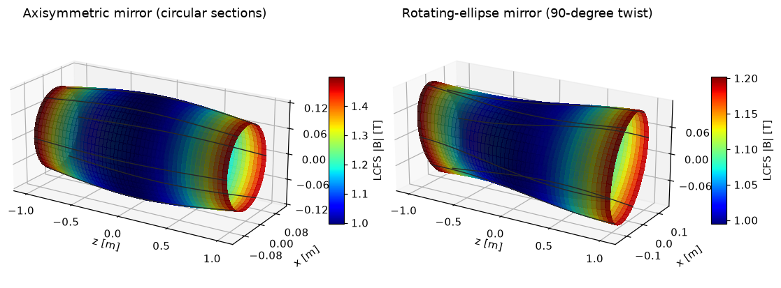
"""Native-spline fixed-boundary mirror equilibria.

Solves the supported rotating-ellipse case, the Agren-Savenko straight
field-line paraxial-accuracy benchmark, and a standard axisymmetric mirror,
then renders the axisymmetric and 90-degree rotating-ellipse solves side by
side in 3-D. The straight field-line mirror is an analytic field that is only
an equilibrium to order ``(a/c)^2``; it is gated on its clean unconstrained
bulk force and on the refinement convergence of that bulk force, and its
elevated end-collar force is the expected boundary layer at the frozen cuts.
"""

from __future__ import annotations

import json
from pathlib import Path
import sys

import jax
import jax.numpy as jnp

REPO_ROOT = Path(__file__).resolve().parents[1]
if str(REPO_ROOT) not in sys.path:
    sys.path.insert(0, str(REPO_ROOT))

from vmex.mirror import (  # noqa: E402
    MirrorBoundary,
    MirrorConfig,
    MirrorResolution,
    MirrorState,
    SplineMirrorBoundary,
    SplineMirrorDiscretization,
    mout_from_result,
    plot_mout,
    solve_fixed_boundary,
    solve_fixed_boundary_from_radius,
    spline_fixed_boundary_adjoint,
    write_mout,
)
from vmex.mirror.analytic import (  # noqa: E402
    AxisymmetricPolynomialMirror,
    RotatingEllipseParaxial,
    StraightFieldLineMirror,
)
from vmex.mirror.output import plot_mirror_3d_pair  # noqa: E402
from vmex.mirror.implicit import spline_fixed_boundary_parameters  # noqa: E402
from vmex.mirror.forces import force_gate_zones  # noqa: E402
from vmex.mirror.splines import initialize_from_cartesian_field  # noqa: E402

# Inputs: edit these constants, then run this file directly.
CASES = ("rotating_ellipse", "straight_field_line")
NS, MPOL, SOURCE_NXI = 7, 6, 17
SPLINE_ELEMENTS = 6
SHAPE_STAGES = (0.0, 0.25, 0.5, 0.75, 1.0)
FTOL = 1.0e-12
MAX_ITERATIONS = 1000
RUN_GRADIENT_CHECK = True
FINITE_DIFFERENCE_STEP = 2.0e-4
STRONG_FORCE_GATE = 5.0e-2
OUTPUT_DIR = Path("results/mirror_fixed_boundary_nonaxisymmetric")

RADIUS = {"rotating_ellipse": 0.12, "straight_field_line": 0.10}
AXIAL_FLUX_DERIVATIVE = {"rotating_ellipse": 0.0072, "straight_field_line": 0.005}
AXISYMMETRIC_RADIUS = 0.12
AXISYMMETRIC_MPOL = 4
AXISYMMETRIC_MIRROR_STRENGTH = 0.5

jax.config.update("jax_enable_x64", True)
OUTPUT_DIR.mkdir(parents=True, exist_ok=True)
config = MirrorConfig(
    resolution=MirrorResolution(ns=NS, mpol=MPOL, nxi=SOURCE_NXI),
    z_min=-1.0,
    z_max=1.0,
    ftol=FTOL,
    max_iterations=MAX_ITERATIONS,
)
source_grid = config.build_grid()
discretization = SplineMirrorDiscretization.build(config, elements=SPLINE_ELEMENTS)
theta = jnp.asarray(source_grid.theta)[:, None]
z = jnp.asarray(source_grid.z)[None, :]


def boundary_for(case: str, stage: float) -> MirrorBoundary:
    """Return one analytic continuation boundary on the source grid."""

    radius = RADIUS[case]
    if case == "rotating_ellipse":
        fixture = RotatingEllipseParaxial(
            half_length=1.0,
            mirror_strength=0.2 * stage,
            elongation=1.0 + 0.5 * stage,
            rotation=0.5 * jnp.pi * stage,
        )
        values = fixture.boundary_radius(radius, theta, z)
    elif case == "straight_field_line":
        fixture = StraightFieldLineMirror(center_field=1.0, axial_scale=2.5)
        values = fixture.boundary_radius(radius, theta, stage * z)
    else:
        raise ValueError(f"unknown mirror case {case!r}")
    return MirrorBoundary.from_radius(values, source_grid)


summaries = {}
for case in CASES:
    initial_boundary = boundary_for(case, 0.0)
    previous_boundary = discretization.fit_boundary(initial_boundary, source_grid)
    coefficient_state = discretization.fit_state(MirrorState.from_boundary(initial_boundary, source_grid), source_grid)
    axial_flux_derivative = AXIAL_FLUX_DERIVATIVE[case]
    stage_iterations = []
    for stage in SHAPE_STAGES:
        final_boundary = discretization.fit_boundary(boundary_for(case, stage), source_grid)
        coefficient_state = discretization.transfer_boundary(coefficient_state, previous_boundary, final_boundary)
        if stage > 0.0:
            if case == "rotating_ellipse":
                fixture = RotatingEllipseParaxial(
                    half_length=1.0,
                    reference_field=2.0 * AXIAL_FLUX_DERIVATIVE[case] / RADIUS[case] ** 2,
                    mirror_strength=0.2 * stage,
                    elongation=1.0 + 0.5 * stage,
                    rotation=0.5 * jnp.pi * stage,
                )
            else:
                fixture = StraightFieldLineMirror(
                    center_field=1.0,
                    axial_scale=2.5 / stage,
                )
            initialized = initialize_from_cartesian_field(
                coefficient_state,
                final_boundary,
                discretization,
                fixture.field,
            )
            coefficient_state = discretization.impose_self_similar_cuts(
                initialized.state,
                final_boundary,
            )
            if case == "straight_field_line":
                axial_flux_derivative = initialized.axial_flux_derivative
        spline_result = solve_fixed_boundary(
            coefficient_state,
            final_boundary,
            discretization,
            config,
            axial_flux_derivative=axial_flux_derivative,
            solve_lambda=True,
            gradient_tolerance=FTOL,
            require_convergence=True,
        )
        coefficient_state = spline_result.coefficient_state
        previous_boundary = final_boundary
        result = spline_result.evaluated
        stage_iterations.append(result.iterations)

    evaluated_boundary = discretization.evaluate_boundary(final_boundary)
    mout_path = write_mout(
        OUTPUT_DIR / f"mout_{case}.nc",
        mout_from_result(
            result,
            discretization.grid,
            config,
            boundary=evaluated_boundary,
            axial_flux_derivative=axial_flux_derivative,
        ),
    )
    plot_mout(mout_path, OUTPUT_DIR, name=case)
    validation = {"lambda_max": float(jnp.max(jnp.abs(coefficient_state.lambda_coefficients)))}
    if case == "rotating_ellipse" and RUN_GRADIENT_CHECK:
        parameters = spline_fixed_boundary_parameters(
            final_boundary,
            axial_flux_derivative=axial_flux_derivative,
        )
        adjoint = spline_fixed_boundary_adjoint(
            spline_result,
            parameters,
            discretization,
            lambda _state, energy: energy.geometry.volume,
            solve_lambda=True,
            rtol=1.0e-9,
        )
        direction = jnp.zeros_like(final_boundary.radius_coefficients)
        direction = direction.at[:, direction.shape[1] // 2].set(1.0e-3)
        predicted = float(jnp.vdot(adjoint.gradient.boundary_coefficients, direction))
        values = []
        for sign in (-1.0, 1.0):
            varied_boundary = SplineMirrorBoundary(
                final_boundary.radius_coefficients + sign * FINITE_DIFFERENCE_STEP * direction
            )
            varied = solve_fixed_boundary(
                discretization.transfer_boundary(
                    spline_result.coefficient_state,
                    final_boundary,
                    varied_boundary,
                ),
                varied_boundary,
                discretization,
                config,
                axial_flux_derivative=axial_flux_derivative,
                solve_lambda=True,
                gradient_tolerance=FTOL,
                require_convergence=True,
            )
            values.append(float(varied.evaluated.energy.geometry.volume))
        finite_difference = (values[1] - values[0]) / (2.0 * FINITE_DIFFERENCE_STEP)
        validation["boundary_gradient_adjoint"] = predicted
        validation["boundary_gradient_finite_difference"] = finite_difference
        validation["boundary_gradient_relative_error"] = abs(predicted - finite_difference) / abs(finite_difference)
        validation["adjoint_relative_residual"] = adjoint.relative_residual
    supported = case == "rotating_ellipse"
    zones = force_gate_zones(result.force)
    # The rotating ellipse is a supported equilibrium and is gated on its
    # all-volume force. The straight field-line mirror is an analytic field
    # that is only an equilibrium to order (a/c)^2, so it is gated on its
    # clean unconstrained bulk force; its elevated end-collar force is the
    # expected boundary layer where the analytic cut profile is frozen.
    status = (
        "supported"
        if supported
        else "paraxial-accuracy benchmark: bulk force gated, cut collar expected"
    )
    summaries[case] = {
        "status": status,
        "stage_iterations": stage_iterations,
        "linear_iterations": result.linear_iterations,
        "final_linear_residual": result.final_linear_residual,
        "variational_max": float(result.variational.maximum),
        "staggered_weak_max": float(result.staggered_weak_force.maximum),
        "strong_force_normalized_rms": zones.all_volume,
        "strong_force_axis_rms": zones.axis_row,
        "strong_force_first_row_rms": zones.first_row,
        "strong_force_bulk_rms": zones.bulk,
        "strong_force_end_collar_rms": zones.end_collar,
        "strong_force_device_normalized_rms": zones.device_all_volume,
        "minor_radius": zones.minor_radius,
        "normalized_divergence_rms": float(result.normalized_divergence_rms),
        "axial_flux_derivative_min": float(jnp.min(jnp.asarray(axial_flux_derivative))),
        "axial_flux_derivative_max": float(jnp.max(jnp.asarray(axial_flux_derivative))),
        **validation,
    }
    assert float(result.variational.maximum) <= FTOL
    assert float(result.normalized_divergence_rms) < 1.0e-12
    if supported:
        assert float(result.staggered_weak_force.maximum) <= 1.1 * FTOL
        assert zones.all_volume < STRONG_FORCE_GATE
    else:
        # Bulk (unconstrained volume) force is the physical equilibrium gate;
        # its refinement convergence is recorded in docs/mirror_geometry.rst.
        assert zones.bulk < STRONG_FORCE_GATE

# Standard axisymmetric mirror through the one-call entry point: the boundary
# is the exact circular flux surface of an analytic vacuum mirror.
axisymmetric_fixture = AxisymmetricPolynomialMirror(
    center_field=1.0,
    half_length=1.0,
    mirror_strength=AXISYMMETRIC_MIRROR_STRENGTH,
)
axisymmetric_config = MirrorConfig(
    resolution=MirrorResolution(ns=NS, mpol=AXISYMMETRIC_MPOL, nxi=SOURCE_NXI),
    z_min=-1.0,
    z_max=1.0,
    ftol=FTOL,
    max_iterations=MAX_ITERATIONS,
)
axisymmetric_grid = axisymmetric_config.build_grid()
axisymmetric_radius = axisymmetric_fixture.boundary_radius(
    AXISYMMETRIC_RADIUS,
    jnp.asarray(axisymmetric_grid.z),
)
axisymmetric_flux_derivative = float(axisymmetric_fixture.poloidal_flux(AXISYMMETRIC_RADIUS, 0.0))
axisymmetric_result = solve_fixed_boundary_from_radius(
    axisymmetric_radius,
    axisymmetric_config,
    elements=SPLINE_ELEMENTS,
    axial_flux_derivative=axisymmetric_flux_derivative,
    solve_lambda=True,
    gradient_tolerance=FTOL,
    require_convergence=True,
)
axisymmetric_evaluated = axisymmetric_result.evaluated
axisymmetric_discretization = SplineMirrorDiscretization.build(axisymmetric_config, elements=SPLINE_ELEMENTS)
axisymmetric_boundary = axisymmetric_discretization.fit_boundary(
    MirrorBoundary.from_radius(axisymmetric_radius, axisymmetric_grid),
    axisymmetric_grid,
)
axisymmetric_mout = write_mout(
    OUTPUT_DIR / "mout_axisymmetric.nc",
    mout_from_result(
        axisymmetric_evaluated,
        axisymmetric_discretization.grid,
        axisymmetric_config,
        boundary=axisymmetric_discretization.evaluate_boundary(axisymmetric_boundary),
        axial_flux_derivative=axisymmetric_flux_derivative,
    ),
)
plot_mout(axisymmetric_mout, OUTPUT_DIR, name="axisymmetric")
summaries["axisymmetric"] = {
    "status": "supported",
    "iterations": axisymmetric_evaluated.iterations,
    "variational_max": float(axisymmetric_evaluated.variational.maximum),
    "staggered_weak_max": float(axisymmetric_evaluated.staggered_weak_force.maximum),
    "strong_force_normalized_rms": float(axisymmetric_evaluated.force.normalized_rms),
    "normalized_divergence_rms": float(axisymmetric_evaluated.normalized_divergence_rms),
    "axial_flux_derivative": axisymmetric_flux_derivative,
    "mirror_ratio": float(1.0 + AXISYMMETRIC_MIRROR_STRENGTH),
}
assert float(axisymmetric_evaluated.variational.maximum) <= FTOL
assert float(axisymmetric_evaluated.staggered_weak_force.maximum) <= 1.1 * FTOL
assert float(axisymmetric_evaluated.force.normalized_rms) < STRONG_FORCE_GATE
assert float(axisymmetric_evaluated.normalized_divergence_rms) < 1.0e-12

# Side-by-side solved 3-D geometry: circular-section axisymmetric mirror on
# the left, the 90-degree rotating ellipse on the right, coloured by LCFS |B|.
pair_figure = plot_mirror_3d_pair(
    axisymmetric_mout,
    OUTPUT_DIR / "mout_rotating_ellipse.nc",
    OUTPUT_DIR,
    titles=(
        "Axisymmetric mirror (circular sections)",
        "Rotating-ellipse mirror (90-degree twist)",
    ),
    name="mirror_fixed_boundary_3d",
)
print(f"Wrote paired fixed-boundary 3-D figure: {pair_figure}")

(OUTPUT_DIR / "summary.json").write_text(json.dumps(summaries, indent=2) + "\n")
print(json.dumps(summaries, indent=2))
Free-boundary mirror beta scan
Two circular end coils drive an open-field equilibrium whose lateral LCFS is
solved jointly with the exterior vacuum. The model is supported through 10%;
the 25% and 50% endpoints are converged but remain validation-only because
their independent force/refinement gates fail. The plots include the
horizontal mirror, coils, cap-to-cap field lines, |B|, pressure,
cross-sections, and force history. The default exterior solve is intentionally
a full/nightly workflow.
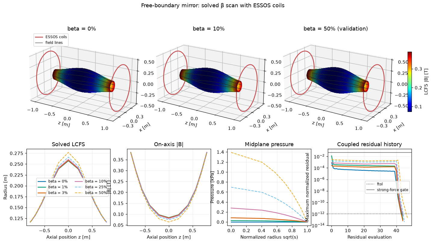
"""Solved two-coil free-boundary mirror beta scan and physics plots.

Run from the repository root with::

    python examples/mirror_free_boundary_beta_scan.py

The first four points are the supported 0--10% validation scan. The last two
are continuation states whose independent force/refinement gates do not pass.
Every curve and surface comes from a coupled
plasma-boundary-vacuum equilibrium solve with residual tolerance ``FTOL``; no
prescribed finite-beta boundary is plotted.
"""

import json
from pathlib import Path
import sys

import jax
import jax.numpy as jnp
import numpy as np

REPO_ROOT = Path(__file__).resolve().parents[1]
if str(REPO_ROOT) not in sys.path:
    sys.path.insert(0, str(REPO_ROOT))

from vmex.mirror import (  # noqa: E402
    MirrorBoundary,
    MirrorConfig,
    MirrorResolution,
    SplineMirrorDiscretization,
    mout_from_result,
    plot_mout,
    solve_beta_scan,
    write_mout,
)
from vmex.mirror.output import (  # noqa: E402
    plot_axisymmetric_beta_scan_summary,
    summarize_axisymmetric_beta_scan,
)
from vmex.mirror.output import (  # noqa: E402
    FreeBoundaryRestart,
    load_free_boundary_restart,
    save_free_boundary_restart,
)

# Inputs: edit these values, then run the file directly.
BETAS = np.asarray([0.0, 0.01, 0.03, 0.10, 0.25, 0.50])
SUPPORTED_BETA_MAX = 0.10
STRONG_FORCE_GATE = 5.0e-2
NS = 7
NXI = 13
SPLINE_ELEMENTS = 7
EXTERIOR_NTHETA = 12
EXTERIOR_ORDER = 6
EXTERIOR_SPECTRAL_SIDE_DENSITY = True
FTOL = 1.0e-12
MAX_ITERATIONS = 2000
Z_MIN, Z_MAX = -0.8, 0.8
# Compact coils sized to the plasma: same vacuum on-axis midplane field as the
# former 0.9 m / 2.0e5 A loops (B(0) ~ 0.0836 T), with a deeper mirror well.
COIL_RADIUS = 0.5
COIL_SEPARATION = 2.0
COIL_CURRENT = 3.72e5
CENTER_RADIUS = 0.25
OUTPUT_DIR = Path("results/mirror_free_boundary_beta_scan")
SAVE_RESTARTS = True
RESTART_FROM = None  # e.g. OUTPUT_DIR / "beta_003p0pct.npz"; then trim BETAS

jax.config.update("jax_enable_x64", True)
OUTPUT_DIR.mkdir(parents=True, exist_ok=True)

coil_dofs = np.zeros((2, 3, 3))
coil_dofs[:, 0, 2] = COIL_RADIUS
coil_dofs[:, 1, 1] = COIL_RADIUS
coil_dofs[:, 2, 0] = np.asarray([-0.5, 0.5]) * COIL_SEPARATION
try:
    from essos.coils import Coils, Curves
    from essos.fields import BiotSavart
except ModuleNotFoundError as error:
    raise ModuleNotFoundError("This example requires ESSOS: pip install -e /path/to/ESSOS") from error

coils = Coils(
    Curves(jnp.asarray(coil_dofs), n_segments=128, nfp=1, stellsym=False),
    jnp.full(2, COIL_CURRENT),
)
biot_savart = BiotSavart(coils)


def external_field(points):
    """Evaluate the ESSOS field on an arbitrary array of Cartesian points."""

    points = jnp.asarray(points)
    return jax.vmap(biot_savart.B)(points.reshape(-1, 3)).reshape(points.shape)


config = MirrorConfig(
    resolution=MirrorResolution(ns=NS, mpol=0, nxi=NXI),
    z_min=Z_MIN,
    z_max=Z_MAX,
    ftol=FTOL,
    max_iterations=MAX_ITERATIONS,
)
source_grid = config.build_grid()
discretization = SplineMirrorDiscretization.build_cgl(config, elements=SPLINE_ELEMENTS)
grid = discretization.grid
initial_restart = None if RESTART_FROM is None else load_free_boundary_restart(RESTART_FROM, discretization)
z = jnp.asarray(grid.z)
coil_z = 0.5 * COIL_SEPARATION
vacuum_axis_field = sum(
    4.0e-7 * jnp.pi * COIL_CURRENT * COIL_RADIUS**2 / (2.0 * (COIL_RADIUS**2 + (z - position) ** 2) ** 1.5)
    for position in (-coil_z, coil_z)
)
center = int(np.argmin(np.abs(grid.z)))
axial_flux_derivative = 0.5 * vacuum_axis_field[center] * CENTER_RADIUS**2
initial_boundary = discretization.fit_boundary(
    MirrorBoundary.from_axis_field(
        axial_flux_derivative,
        vacuum_axis_field,
        grid,
    ),
    source_grid,
)
print(f"Solving {BETAS.size} beta points at ns={NS}, nxi={NXI}, ftol={FTOL:.0e}")
results = solve_beta_scan(
    initial_boundary,
    discretization,
    config,
    external_field,
    jnp.asarray(BETAS),
    axial_flux_derivative=axial_flux_derivative,
    reference_field=float(vacuum_axis_field[center]),
    initial_restart=initial_restart,
    exterior_ntheta=EXTERIOR_NTHETA,
    exterior_order=EXTERIOR_ORDER,
    exterior_spectral_side_density=EXTERIOR_SPECTRAL_SIDE_DENSITY,
)
gamma = np.asarray(coils.gamma)
if SAVE_RESTARTS:
    for beta, result in zip(BETAS, results, strict=True):
        label = f"beta_{100 * beta:05.1f}pct".replace(".", "p")
        save_free_boundary_restart(OUTPUT_DIR / label, FreeBoundaryRestart.from_result(result))
for beta, result in zip(BETAS, results, strict=True):
    label = f"beta_{100 * beta:05.1f}pct".replace(".", "p")
    write_mout(
        OUTPUT_DIR / f"mout_mirror_{label}.nc",
        mout_from_result(
            result,
            grid,
            config,
            axial_flux_derivative=axial_flux_derivative,
            coil_xyz=gamma,
        ),
    )
diagnostics = summarize_axisymmetric_beta_scan(
    results,
    jnp.asarray(BETAS),
    grid,
    reference_field=float(vacuum_axis_field[center]),
)


summary = [
    {key: float(value) for key, value in vars(item).items()}
    | {
        "variational_max": float(result.variational_max),
        "pointwise_force_rms": float(result.plasma_force.normalized_rms),
        "supported_lane": bool(
            item.requested_beta <= SUPPORTED_BETA_MAX
            and float(result.plasma_force.normalized_rms) < STRONG_FORCE_GATE
        ),
        "model_supported_beta_range": bool(item.requested_beta <= SUPPORTED_BETA_MAX),
        "passes_strong_force_gate": bool(
            float(result.plasma_force.normalized_rms) < STRONG_FORCE_GATE
        ),
    }
    for item, result in zip(diagnostics, results, strict=True)
]
(OUTPUT_DIR / "beta_scan_summary.json").write_text(json.dumps(summary, indent=2) + "\n")
for row in summary:
    if row["model_supported_beta_range"]:
        assert row["passes_strong_force_gate"], f"supported beta point failed the force gate: {row}"

middle_beta = min(0.10, 0.5 * float(BETAS[-1]))
display_indices = sorted({0, int(np.argmin(np.abs(BETAS - middle_beta))), len(BETAS) - 1})
for index in display_indices:
    label = f"beta_{100 * BETAS[index]:05.1f}pct".replace(".", "p")
    plot_mout(
        OUTPUT_DIR / f"mout_mirror_{label}.nc",
        OUTPUT_DIR,
        name=f"mirror_{label}",
    )

mirror_ratio = float(jnp.max(vacuum_axis_field) / vacuum_axis_field[center])
radius_expansion = 100.0 * (summary[-1]["center_radius"] / summary[0]["center_radius"] - 1.0)
field_reduction = 100.0 * (1.0 - summary[-1]["diamagnetic_field_ratio"])
final_gate = (
    "its independent force gate fails"
    if not summary[-1]["passes_strong_force_gate"]
    else "beyond the supported model range"
)
caption = (
    f"Two ESSOS loops (radius {COIL_RADIUS} m at z = +/-{0.5 * COIL_SEPARATION} m, "
    f"{COIL_CURRENT:.3g} A each) give vacuum B(0) = {float(vacuum_axis_field[center]):.4f} T and "
    f"on-grid mirror ratio {mirror_ratio:.2f}. Betas through {100 * SUPPORTED_BETA_MAX:g}% pass the "
    f"strong-force gate; the {100 * float(BETAS[-1]):g}% validation continuation expands the center radius by "
    f"{radius_expansion:.2f}% and lowers the on-axis field by {field_reduction:.2f}% ({final_gate})."
)
composite = plot_axisymmetric_beta_scan_summary(
    [
        (
            f"beta = {100 * beta:g}%",
            OUTPUT_DIR / f"mout_mirror_{f'beta_{100 * beta:05.1f}pct'.replace('.', 'p')}.nc",
            bool(row["supported_lane"]),
        )
        for beta, row in zip(BETAS, summary, strict=True)
    ],
    OUTPUT_DIR,
    display=tuple(display_indices),
    strong_force_gate=STRONG_FORCE_GATE,
)

# The figure stays clean (short title + panel labels only); the coil geometry,
# vacuum field, mirror ratio, and beta observables are reported here and in
# docs/mirror_geometry.rst.
print(caption)
print(json.dumps(summary, indent=2))
print(f"Wrote solved-state 3D, cross-section, |B|, and summary plots in {OUTPUT_DIR}")
print(f"Wrote beta-scan composite figure: {composite}")
Periodic stellarator-mirror hybrid
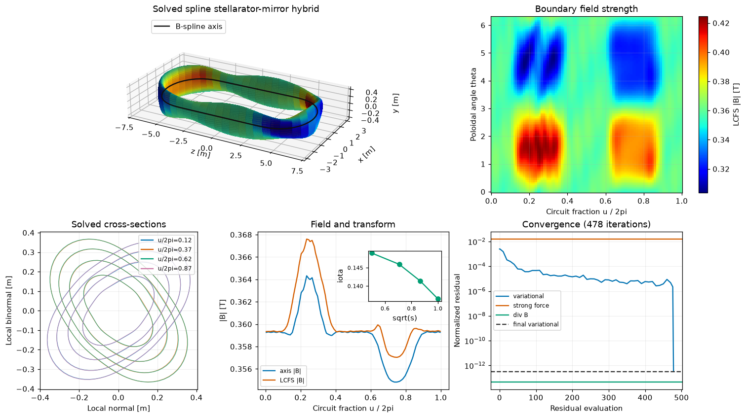
Join two exactly straight mirror legs with two curved periodic B-spline
returns. The elliptical section rotates by 90 degrees through each return, and
a finite current produces visible field-line pitch. The example performs the
fixed-boundary equilibrium solve before plotting its LCFS |B|, actual
field lines, cross-sections, iota, and convergence diagnostics. Its present
coarse strong-force residual is displayed as a failed validation gate.
"""Solve and plot a periodic B-spline stellarator-mirror hybrid."""

from __future__ import annotations

import json
from pathlib import Path
import sys

import jax

REPO_ROOT = Path(__file__).resolve().parents[1]
if str(REPO_ROOT) not in sys.path:
    sys.path.insert(0, str(REPO_ROOT))

from vmex.mirror import (
    MirrorConfig,
    MirrorResolution,
    build_stellarator_mirror_hybrid,
    plot_stellarator_mirror_hybrid,
    solve_fixed_boundary,
    trace_closed_field_line,
)

# Inputs: edit these values, then run this file directly.
NS, MPOL = 5, 4
SPLINE_COEFFICIENTS = 32
SPLINE_QUADRATURE_ORDER = 3
STRAIGHT_LENGTH = 8.0
RETURN_RADIUS = 2.5
SEMI_MAJOR = 0.45
SEMI_MINOR = 0.25
# Turn the elliptical cross-section continuously around the closed circuit by
# this many full 2*pi turns (a genuine rotating-ellipse section) on top of the
# return-only 90-degree rotation. The legs keep an exactly straight axis; only
# the ellipse they carry rotates. Two turns lifts the transform from the
# return-only iota=0.085 to iota=0.141 at s=0.75 here. Set 0 for the legacy
# return-only rotation.
SECTION_TURNS = 2
AXIAL_FLUX_DERIVATIVE = 0.02
CURRENT_DERIVATIVE = 0.002
FTOL = 1.0e-12
MAX_ITERATIONS = 1000
OUTPUT_DIR = Path("results/stellarator_mirror_hybrid")

jax.config.update("jax_enable_x64", True)
OUTPUT_DIR.mkdir(parents=True, exist_ok=True)

resolution = MirrorResolution(ns=NS, mpol=MPOL, nxi=4)
config = MirrorConfig(
    resolution=resolution,
    ftol=FTOL,
    max_iterations=MAX_ITERATIONS,
)
setup = build_stellarator_mirror_hybrid(
    resolution,
    coefficient_count=SPLINE_COEFFICIENTS,
    straight_length=STRAIGHT_LENGTH,
    return_radius=RETURN_RADIUS,
    semi_major=SEMI_MAJOR,
    semi_minor=SEMI_MINOR,
    section_turns=SECTION_TURNS,
    axial_flux_derivative=AXIAL_FLUX_DERIVATIVE,
    quadrature_order=SPLINE_QUADRATURE_ORDER,
)
result = solve_fixed_boundary(
    setup.initial_state,
    setup.boundary,
    setup.discretization,
    config,
    axial_flux_derivative=AXIAL_FLUX_DERIVATIVE,
    current_derivative=CURRENT_DERIVATIVE,
    solve_lambda=True,
    axis=setup.axis,
    require_convergence=True,
)
figure = plot_stellarator_mirror_hybrid(result, setup, OUTPUT_DIR)
field_line = trace_closed_field_line(
    result.evaluated.energy.field,
    setup.discretization,
    radial_index=NS - 2,
    turns=2,
)
summary = {
    "converged": result.evaluated.converged,
    "iterations": result.evaluated.iterations,
    "variational_max": float(result.evaluated.variational.maximum),
    "staggered_weak_max": float(result.evaluated.staggered_weak_force.maximum),
    "strong_force_normalized_rms": float(result.evaluated.force.normalized_rms),
    "strong_force_axis_rms": float(result.evaluated.force.axis_normalized_rms),
    "strong_force_first_row_rms": float(result.evaluated.force.first_row_normalized_rms),
    "strong_force_bulk_rms": float(result.evaluated.force.bulk_normalized_rms),
    "strong_force_components": [float(value) for value in result.evaluated.force.component_rms],
    "normalized_divergence_rms": float(result.evaluated.normalized_divergence_rms),
    "volume": float(result.evaluated.energy.geometry.volume),
    "axis_length": float(setup.axis.arc_length),
    "axis_closure_error": float(setup.axis.closure_error),
    "frame_closure_error": float(setup.axis.frame_closure_error),
    "section_turns": SECTION_TURNS,
    "iota_at_s_0p75": float(field_line.iota),
    "figure": str(figure),
}
(OUTPUT_DIR / "summary.json").write_text(json.dumps(summary, indent=2) + "\n")
print(json.dumps(summary, indent=2))
Independent Pleiades reference
The resolution-qualified two-coil beta trend is independently regenerated
with Pleiades at pinned commit 0161abb3. Set PLEIADES_ROOT at the top;
the script writes ignored review output and never silently replaces the bundled
CSV benchmark.
"""Regenerate the independent Pleiades two-coil mirror reference.

Set ``PLEIADES_ROOT`` below to a checkout of
``github.com/eepeterson/pleiades`` at commit
``0161abb3e9a1d85143c650f068ec524d672fc9ab``, then run this file directly.
The output belongs under ignored ``results/``; review it before deliberately
updating ``examples/data/pleiades_two_coil_beta_reference.csv``.
"""

import collections
import collections.abc
import contextlib
import io
from pathlib import Path
import sys

import matplotlib
import numpy as np

matplotlib.use("Agg")
import matplotlib.pyplot as plt  # noqa: E402

# Inputs
PLEIADES_ROOT = Path("/path/to/pleiades")
RESOLUTIONS = ((31, 61), (41, 81), (51, 101))
BETAS = (0.01, 0.03, 0.10)
OUTPUT_DIR = Path("results/pleiades_mirror_reference")

if not (PLEIADES_ROOT / "pleiades" / "eq_solve.py").is_file():
    raise SystemExit("Set PLEIADES_ROOT at the top of this file to a Pleiades checkout")
sys.path.insert(0, str(PLEIADES_ROOT))
collections.Iterable = collections.abc.Iterable  # Pleiades 2021 compatibility with Python 3.10+

from pleiades import ArbitraryPoints, RectMesh, compute_equilibrium  # noqa: E402
from pleiades.analysis import get_gpsi  # noqa: E402
from pleiades.fields import compute_greens  # noqa: E402

MU0 = 4.0e-7 * np.pi
rows = []
for nr, nz in RESOLUTIONS:
    mesh = RectMesh(rmin=0.0, rmax=0.5, nr=nr, zmin=-0.8, zmax=0.8, nz=nz)
    radius, z = mesh.R, mesh.Z
    coils = ArbitraryPoints(np.asarray([[0.9, -1.0], [0.9, 1.0]]), current=2.0e5)
    coils.mesh = mesh
    vacuum_flux = np.asarray(coils.psi()).reshape(radius.shape)
    center = int(np.argmin(np.abs(z[:, 0])))
    vacuum_axis_field = float(np.asarray(coils.BZ()).reshape(radius.shape)[center, 0])
    with contextlib.redirect_stdout(io.StringIO()):
        plasma_green = get_gpsi(radius, z)
    for beta in BETAS:
        pressure0 = beta * vacuum_axis_field**2 / (2.0 * MU0)

        def pressure(radial_position, pressure0=pressure0):
            return pressure0 * (1.0 - (radial_position / 0.25) ** 2) if radial_position < 0.25 else 0.0

        output = io.StringIO()
        with contextlib.redirect_stdout(output):
            _, plasma_currents, _ = compute_equilibrium(
                radius,
                z,
                pressure,
                vacuum_flux,
                plasma_green,
                tol=1.0e-10,
                maxiter=400,
                relax=0.9,
            )
        trace = output.getvalue().strip().splitlines()
        iterations, iteration_error = int(trace[-2]), float(trace[-1])
        current_loops = np.column_stack([radius.ravel(), z.ravel(), plasma_currents.ravel()])
        plasma_axis_field = float(compute_greens(current_loops, np.asarray([[0.0, 0.0]]))[2][0])
        axis_field = vacuum_axis_field + plasma_axis_field
        rows.append((nr, nz, beta, iterations, iteration_error, vacuum_axis_field, axis_field, axis_field / vacuum_axis_field))

OUTPUT_DIR.mkdir(parents=True, exist_ok=True)
data = np.asarray(rows)
header = "nr,nz,beta,iterations,iteration_error,vacuum_axis_field_T,axis_field_T,field_ratio"
np.savetxt(OUTPUT_DIR / "pleiades_two_coil_beta_reference.csv", data, delimiter=",", header=header, comments="")
fig, ax = plt.subplots(figsize=(6.2, 4.2), constrained_layout=True)
for nr, nz in RESOLUTIONS:
    selected = data[(data[:, 0] == nr) & (data[:, 1] == nz)]
    ax.plot(100 * selected[:, 2], selected[:, -1], "o-", lw=1.8, label=f"{nr}x{nz}")
ax.plot(100 * data[: len(BETAS), 2], np.sqrt(1.0 - data[: len(BETAS), 2]), "k--", label=r"$\sqrt{1-\beta}$")
ax.set(xlabel="Central beta [%]", ylabel=r"$B(\beta)/B_{vac}$", title="Pleiades two-coil reference convergence")
ax.grid(alpha=0.22)
ax.legend()
fig.savefig(OUTPUT_DIR / "pleiades_two_coil_beta_reference.png", dpi=180)
print(data)
Optimization
The examples/optimization/ gallery drives a circular torus to precise
quasisymmetric (QA, QH, QP) and quasi-isodynamic (QI) configurations with
gradient-based least squares — user-authored (function, target, weight)
objective terms with implicit-differentiation gradients
(jac="implicit"). See Objectives library for the full objective library
(quasisymmetry and omnigenity residuals, Redl bootstrap, ballooning
stability, turbulence proxies, scalar targets) and Optimization and differentiability for
the differentiation machinery and the measured campaign timings.
Single-call ESS optimization (recommended)
The recommended pattern is one least_squares call with all the
boundary harmonics released at once and Exponential Spectral Scaling
(use_ess=True) ordering them through the trust region — no
max_mode continuation loop. Measured: precise QA (QS 7.2e-6) in
14.5 minutes on a CPU.
#!/usr/bin/env python
"""Precise QA in ONE least-squares call: no mode-continuation ladder, just ESS.

The staged examples (``QA_optimization.py`` etc.) walk ``max_mode`` 1 -> 5 so
the optimizer settles the long-wavelength shape before the fine harmonics are
released.  This script shows the alternative that makes the ladder
unnecessary: hand the optimizer *all* the max_mode-5 boundary harmonics at
once and let **Exponential Spectral Scaling** (``use_ess=True``) do the
ordering — the trust-region radius of each dof is scaled by
``exp(-alpha * max(|m|, |n|))``, so high harmonics move on exponentially
shorter leashes and the optimizer explores the same coarse-to-fine hierarchy
implicitly, in a single stage.

Physics setup is identical to ``QA_optimization.py`` (nfp=2 vacuum QA from a
near-circular torus, quasisymmetry + aspect + iota targets, implicit adjoint
gradients).  Measured 2026-07-12 on the office 36-core CPU (memo + block
Jacobian + perturbation warm start):

    seed QS 2.043e-01 -> final QS 7.155e-06 (aspect 6.000, iota 0.420)
    in ONE call, 868 s (14.5 min) — vs 1532 s for the staged 1->5 ladder
    reaching 3.7e-07.  Same precision class, ~1.8x faster, no ladder.
"""

import dataclasses
import os
from pathlib import Path

import numpy as np

import vmex as vj
from vmex import optimize as opt

# --------------------------- parameters ------------------------------------
INPUT_FILE = Path(__file__).resolve().parents[1] / "data" / "input.minimal_seed_nfp2"
OUT_DIR = Path("output_QA_optimization_ess")
QS_SURFACES = np.linspace(0.1, 1.0, 10)
HELICITY_M, HELICITY_N = 1, 0             # QA: |B| = |B|(s, theta)
ASPECT_TARGET = 6.0
IOTA_TARGET = 0.42
SEED_PERTURBATION = 0.01                  # helical kick off the axisymmetric saddle
MAX_MODE = 5                              # ALL harmonics at once — no ladder
ESS_ALPHA = 0.7                           # trust-region decay per harmonic order
MAX_NFEV = 4000                           # single-stage budget (~2 ladder stages)
FTOL = 1e-8
JAC = "implicit"
if os.environ.get("VMEX_EXAMPLES_CI") == "1":  # smoke-test budget
    MAX_MODE, MAX_NFEV, FTOL = 2, 4, 1e-4

# --------------------------- seed equilibrium ------------------------------
inp = vj.VmecInput.from_file(INPUT_FILE)
rbc, zbs = inp.rbc.copy(), inp.zbs.copy()
rbc[inp.ntor + 1, 1] += SEED_PERTURBATION  # break the axisymmetric tie
zbs[inp.ntor + 1, 1] += SEED_PERTURBATION
inp = dataclasses.replace(inp, rbc=rbc, zbs=zbs)
qs = opt.QuasisymmetryRatioResidual(QS_SURFACES, HELICITY_M, HELICITY_N)


def report(tag, eq):
    total = float(qs.total(eq))
    print(f"[{tag}] QS total = {total:.6e}, "
          f"aspect = {float(opt.aspect_ratio(eq.state, eq.runtime)):.4f}, "
          f"mean iota = {float(opt.mean_iota(eq.state, eq.runtime)):.4f}")
    return total


qs_seed = report("seed", opt.solve_equilibrium(inp))

# --------------------------- objective (user-authored) ---------------------
objective_terms = [
    (qs, 0.0, 1.0),
    (opt.aspect_ratio, ASPECT_TARGET, 1.0),
    (opt.mean_iota, IOTA_TARGET, 1.0),
]

# --------------------------- ONE least-squares call ------------------------
ndofs = len(opt.boundary_dof_names(inp, MAX_MODE))
print(f"\nsingle stage: max_mode = {MAX_MODE} ({ndofs} boundary dofs), "
      f"ESS alpha = {ESS_ALPHA}")
result = opt.least_squares(
    objective_terms, inp, max_mode=MAX_MODE, jac=JAC,
    use_ess=True, ess_alpha=ESS_ALPHA,      # <-- the ladder-replacement
    verbose=1, max_nfev=MAX_NFEV, ftol=FTOL, xtol=1e-10,
)
inp = result.input

# --------------------------- final results ---------------------------------
qs_final = qs_seed
if result.equilibrium is not None:
    qs_final = report("final", result.equilibrium)
print(f"\nQS total: seed {qs_seed:.3e} -> final {qs_final:.3e} "
      f"(one call, no max_mode ladder)")
OUT_DIR.mkdir(parents=True, exist_ok=True)
inp.to_indata(OUT_DIR / "input.QA_ess_optimized")
if result.equilibrium is not None:
    wout_path = vj.write_wout(OUT_DIR / "wout_QA_ess_optimized.nc",
                              result.equilibrium.wout)
    print(f"wrote {wout_path}")
QI_optimization_ess.py is the quasi-isodynamic analogue: the traceable
Goodman constructed-QI residual (QIResidual)
plus practical targets, one call at max_mode = 6 (25x residual
reduction in 17.3 minutes).
Staged max_mode continuation
The classic ladder — one least-squares stage per max_mode, each seeded
with the previous stage’s boundary — remains available and is what
QA_optimization.py, QH_optimization.py, QP_optimization.py, and
QI_optimization.py run (QI with a quasi-poloidal basin stage first).
It reaches the same precision class as the single-call pattern at roughly
twice the wall time; the scripts stay side by side so the comparison is
reproducible.
#!/usr/bin/env python
"""Precise quasi-axisymmetry (QA) from a circular torus, nfp=2.

Mirrors simsopt's ``QH_fixed_resolution.py`` example: build an equilibrium,
write the objective yourself as ``(function, target, weight)`` terms —
here the Landreman-Paul QA recipe, the quasisymmetry ratio residual on a
set of surfaces plus aspect-ratio and mean-iota targets — and hand it to one
least-squares call per continuation stage.  The decision variables are the
boundary Fourier coefficients RBC/ZBS up to ``max_mode``, staged 1 -> 5,
with Exponential Spectral Scaling (ESS) of the trust region and implicit
(adjoint) gradients: no finite differences, no MPI.

The seed (``input.minimal_seed_nfp2``) is a circular torus, R0 = 1 m,
a = 0.2 m — exactly axisymmetric, so the QS term starts at ~0 and the iota
target pulls the boundary into three dimensions.

Runtime is dominated by the one-time implicit-Jacobian XLA compile per
continuation stage (the warm forward solve itself is ~0.9 s); each stage
then stops early at ftol.  Achieved 2026-07-10 on an office RTX A4000 GPU
at this script's default staged budget with JAC="implicit" + ESS: the QS
ratio residual total falls 2.043e-01 (circular seed) -> 9.82e-03
(max_mode=1) -> 1.70e-04 (max_mode=2) -- >3 orders of magnitude, i.e.
*precise* QA -- with aspect 6.000 and mean iota 0.420 both on target
(max_mode 3-5 polish further).  Per-stage wall was ~13 min (max_mode=1,
compile-bound) and ~21 min (max_mode=2).  A CPU run reaches the same
optimum: the cold forward solve is ~2x faster than the GPU (13 vs 27 s)
because this small solve is a host callback that the GPU does not help.
"""

import dataclasses
import os
from pathlib import Path

import numpy as np

import vmex as vj
from vmex import optimize as opt

# --------------------------- parameters ------------------------------------
INPUT_FILE = Path(__file__).resolve().parents[1] / "data" / "input.minimal_seed_nfp2"
OUT_DIR = Path("output_QA_optimization")
QS_SURFACES = np.linspace(0.1, 1.0, 10)   # surfaces for the QS ratio residual
HELICITY_M, HELICITY_N = 1, 0             # QA: |B| = |B|(s, theta)
ASPECT_TARGET = 6.0
IOTA_TARGET = 0.42                        # mean rotational transform
SEED_PERTURBATION = 0.01                  # helical kick, see below
MAX_MODE_SCHEDULE = (1, 2, 3, 4, 5)       # boundary-harmonic continuation
MAX_NFEV = 2000                           # trial-boundary budget per stage
FTOL = 1e-6                               # per-stage convergence tolerance
JAC = "implicit"                          # adjoint gradients; None = finite diff
if os.environ.get("VMEX_EXAMPLES_CI") == "1":  # smoke-test budget
    MAX_MODE_SCHEDULE, MAX_NFEV, FTOL = (1,), 4, 1e-4

# --------------------------- seed equilibrium ------------------------------
inp = vj.VmecInput.from_file(INPUT_FILE)   # plain &INDATA parsing
# The exact circular torus is a saddle point: with zero current the
# rotational transform is produced by 3D shaping at *second* order, so its
# gradient vanishes there.  A small RBC/ZBS(n=1, m=1) kick breaks the tie
# (this replaces the seed-preconditioner machinery of the old examples).
rbc, zbs = inp.rbc.copy(), inp.zbs.copy()
rbc[inp.ntor + 1, 1] += SEED_PERTURBATION
zbs[inp.ntor + 1, 1] += SEED_PERTURBATION
inp = dataclasses.replace(inp, rbc=rbc, zbs=zbs)
eq = opt.solve_equilibrium(inp)
qs = opt.QuasisymmetryRatioResidual(QS_SURFACES, HELICITY_M, HELICITY_N)


def report(tag, eq):
    """User-side progress metric: the wout-engine QS total + scalar targets."""
    total = float(qs.total(eq))
    aspect = float(opt.aspect_ratio(eq.state, eq.runtime))
    iota = float(opt.mean_iota(eq.state, eq.runtime))
    print(f"[{tag}] QS total = {total:.6e}, aspect = {aspect:.4f}, "
          f"mean iota = {iota:.4f}")
    return total


qs_seed = report("seed", eq)

# --------------------------- objective (user-authored) ----------------------
objective_terms = [
    (qs, 0.0, 1.0),                       # quasisymmetry ratio residual
    (opt.aspect_ratio, ASPECT_TARGET, 1.0),
    (opt.mean_iota, IOTA_TARGET, 10.0),
    # Extra physics terms, CI-tested (tests/test_examples.py runs
    # them uncommented).  magnetic_well works with JAC="implicit"; d_merc and
    # l_grad_b are wout-engine (host) objectives -> set JAC = None for those.
    # (opt.magnetic_well, 0.05, 1.0),
    # (lambda eq: np.minimum(opt.d_merc(eq)[2:-1], 0.0), 0.0, 100.0),
    # (lambda eq: max(1.0 / opt.l_grad_b(eq) - 1.0 / 0.35, 0.0), 0.0, 1.0),
    # Turbulence proxies (plan R26h.h4; optional dep: pip install spectraxgk;
    # gates in tests/test_turbulence.py).  SPECTRAX-GK linear ITG growth rate
    # (traceable -> works with JAC="implicit" or JAC=None) and quasilinear
    # heat-flux proxy (eigenvector-weighted -> JAC=None only) on a core flux
    # tube:
    #   from vmex.core import turbulence as turb
    # (turb.turbulent_growth_rate, 0.0, 1.0),
    # (turb.quasilinear_flux_proxy, 0.0, 0.1),
]

# --------------------------- staged optimization ----------------------------
for max_mode in MAX_MODE_SCHEDULE:
    ndofs = len(opt.boundary_dof_names(inp, max_mode))
    print(f"\n===== stage max_mode = {max_mode} ({ndofs} boundary dofs) =====")
    result = opt.least_squares(
        objective_terms, inp, max_mode=max_mode, jac=JAC,
        use_ess=True, verbose=1, max_nfev=MAX_NFEV, ftol=FTOL, xtol=1e-10,
    )
    inp = result.input                     # warm-start the next stage
    if result.equilibrium is not None:
        report(f"stage {max_mode}", result.equilibrium)

# --------------------------- final results ---------------------------------
eq = result.equilibrium or opt.solve_equilibrium(inp)
qs_final = report("final", eq)
print(f"\nQS total: seed {qs_seed:.3e} -> final {qs_final:.3e}")
print("optimized boundary (largest coefficients):")
names = opt.boundary_dof_names(inp, MAX_MODE_SCHEDULE[-1])
values = opt.pack_boundary(inp, MAX_MODE_SCHEDULE[-1])
for k in np.argsort(-np.abs(values))[:8]:
    print(f"  {names[k]:>10s} = {values[k]:+.6f}")

OUT_DIR.mkdir(parents=True, exist_ok=True)
inp.to_indata(OUT_DIR / "input.QA_optimized")               # optimized deck
wout_path = vj.write_wout(OUT_DIR / "wout_QA_optimized.nc", eq.wout)
print(f"wrote {OUT_DIR / 'input.QA_optimized'}\nwrote {wout_path}")
for key, path in vj.plot_wout(wout_path, OUT_DIR).items():  # figures
    print(f"wrote {path}")
These are the heaviest examples (hundreds to thousands of solves) and are exercised in the nightly CI run.
Self-consistent bootstrap current
A different loop: instead of reshaping the boundary, regenerate the current
profile until it is consistent with the bootstrap current the plasma itself
drives. QA_bootstrap_selfconsistent.py (and its sibling
QH_bootstrap_selfconsistent.py)
reproduces the quasi-axisymmetric configuration of Landreman–Buller–Drevlak
(arXiv:2205.02914): it erases the deck’s current profile and lets the
fixed-boundary Picard loop
self_consistent_bootstrap() rebuild it from the
Redl formula, converging to the paper’s mismatch f_boot = 2e-6 in a
handful of hot-restarted iterations. The physics of the Redl closure is on
Confinement physics: quasisymmetry, omnigenity, stability.
#!/usr/bin/env python
"""Bootstrap-self-consistent QA (nfp=2, aspect 6, beta=2.5%) of arXiv:2205.02914.

Reproduces the quasi-axisymmetric configuration with self-consistent bootstrap
current of Landreman, Buller & Drevlak, Phys. Plasmas 29, 082501 (2022),
arXiv:2205.02914, from the paper's Zenodo data archive: load the published
boundary + pressure deck, *erase* the current profile (CURTOR = 0, flat I'),
and let the fixed-boundary Picard loop ``self_consistent_bootstrap`` regenerate
it from the Redl formula [Redl et al., Phys. Plasmas 28, 022502 (2021)] with
the paper's kinetic profiles ne = 2.38e20*(1 - s^5) m^-3, Te = Ti =
9.45 keV*(1 - s), Zeff = 1 (the deck's pressure is exactly e*(ne*Te + ni*Ti)).
The recovered profile is checked against two *stored* Zenodo curves: the
published equilibrium's own ``jdotb`` and the paper's SFINCS drift-kinetic
benchmark.  Achieved 2026-07-12 (full mode: deck mpol=16/ntor=12,
ns 13->25->51, ~2 min on CPU): 7 Picard iterations to the paper's mismatch
f_boot = 2.0e-06, I_p = -2.773 MA vs the published CURTOR = -2.721 MA (1.9%),
<J.B> vs the published profile 1.7% RMS, Redl vs SFINCS 3.4% RMS (s in
[0.1, 0.9]).  Needs the Zenodo dataset on disk (default path as in
tests/test_bootstrap.py; override with VMEX_ZENODO_2205_02914); run the
sibling ``QH_bootstrap_selfconsistent.py`` too — whichever finishes second
also assembles the combined two-panel ``readme_bootstrap.png``.
"""

import dataclasses
import os
from pathlib import Path

import numpy as np

import vmex as vj
from vmex.core import bootstrap as bs

# --------------------------- parameters ------------------------------------
ZENODO = Path(os.environ.get(
    "VMEX_ZENODO_2205_02914",
    "/Users/rogerio/local/"
    "20220708-01-zenodo_for_QS_optimization_with_self_consistent_bootstrap_current"))
CONFIG_DIR = ZENODO / "configurations" / "QA_aspect6_beta2.5"
DECK = CONFIG_DIR / "input.QA_beta0p025_iota0p42_dreopt_HIGHERRES_2022-04-15"
WOUT_PUB = CONFIG_DIR / "wout_QA_beta0p025_iota0p42_dreopt_HIGHERRES_2022-04-15.nc"
TAG, TITLE = "QA", "QA   nfp=2, aspect 6, beta=2.5%"
N0, T0 = 2.38e20, 9.45e3        # ne = N0*(1-s^5) [1/m^3], Te = Ti = T0*(1-s) [eV]
HELICITY_N = 0                  # quasi-axisymmetry: |B| = |B|(s, theta)
NS_ARRAY = [13, 25, 51]         # radial ladder (published deck ran to ns=201)
MAX_MODE = None                 # boundary truncation; None = deck resolution
N_ITER, TOL = 10, 1e-3          # Picard budget / I'(s) convergence tolerance
OUT_DIR = Path(f"output_{TAG}_bootstrap_selfconsistent")
if os.environ.get("VMEX_EXAMPLES_CI") == "1":   # smoke-test budget
    NS_ARRAY, MAX_MODE, N_ITER = [13, 25], 6, 2

# The paper's SFINCS (drift-kinetic) benchmark for this configuration, verbatim
# from the Zenodo archive (calculations/figure16); <J.B> [T*A/m^2] on S_EVAL.
S_EVAL = np.linspace(0.02, 0.98, 49)
JDOTB_SFINCS = np.array([
    -916072.12427159, -1324379.20239041, -1544842.87066177, -1675100.6950393, -1762875.6278957, -1827560.97417256,
    -1880517.17309354, -1928408.68312639, -1971292.60356815, -2011759.56920981, -2050031.37024243, -2086385.68422913,
    -2119386.52863304, -2164137.94238967, -2197863.37997822, -2230019.79294978, -2261905.54946878, -2293165.69287045,
    -2323325.83117452, -2352275.13844983, -2381759.96354804, -2408715.82651757, -2433654.28403962, -2455955.22781949,
    -2472835.34373194, -2488148.99860227, -2495986.79022978, -2503389.96325646, -2501058.43950896, -2491407.99615351,
    -2472708.55046093, -2443912.83281386, -2403701.54442513, -2350881.90658299, -2284258.32067799, -2200345.82186852,
    -2103076.26667622, -1987909.48731683, -1855576.01579721, -1703294.32318193, -1535039.37514875, -1350214.75153689,
    -1150828.1176048, -946732.17479023, -711961.96764062, -494943.12151168, -295163.49102646, -133610.01315949,
    -28448.25026866])

# --------------------------- published deck, current erased -----------------
if not DECK.is_file():
    raise SystemExit(f"Zenodo dataset not found at {ZENODO}\n"
                     "set VMEX_ZENODO_2205_02914 to its root directory")
inp_pub = vj.VmecInput.from_file(DECK)      # boundary + pressure + spline current

def truncate_boundary(inp, max_mode):
    """Drop boundary/axis harmonics above ``max_mode`` (CI-budget resolution)."""
    if max_mode is None or max_mode + 1 >= inp.mpol:
        return inp
    m, nt = max_mode, inp.ntor
    rbc = np.zeros((2 * m + 1, m + 1)); zbs = np.zeros((2 * m + 1, m + 1))
    for n in range(-m, m + 1):
        rbc[n + m], zbs[n + m] = inp.rbc[n + nt, :m + 1], inp.zbs[n + nt, :m + 1]
    return dataclasses.replace(
        inp, mpol=m + 1, ntor=m, rbc=rbc, zbs=zbs, rbs=None, zbc=None, raxis_s=None,
        raxis_c=np.asarray(inp.raxis_c)[:m + 1], zaxis_s=np.asarray(inp.zaxis_s)[:m + 1],
        zaxis_c=None)

inp = dataclasses.replace(
    truncate_boundary(inp_pub, MAX_MODE),
    ns_array=NS_ARRAY, ftol_array=[1e-11] * len(NS_ARRAY),
    niter_array=[2000] + [4000] * (len(NS_ARRAY) - 1),
    # erase the published (already self-consistent) current profile:
    ncurr=1, pcurr_type="power_series", ac=np.concatenate([[1.0], np.zeros(20)]),
    curtor=0.0)

# --------------------------- Picard to self-consistency ---------------------
profiles = bs.KineticProfiles(ne_coeffs=N0 * np.array([1, 0, 0, 0, 0, -1.0]),
                              Te_coeffs=T0 * np.array([1, -1.0]),
                              Ti_coeffs=T0 * np.array([1, -1.0]))
res = bs.self_consistent_bootstrap(inp, profiles, HELICITY_N, n_iter=N_ITER, tol=TOL,
                                   s_eval=S_EVAL, verbose=True)
eq, f_boot = res.equilibrium, res.history[-1]["f_boot"]

# --------------------------- compare with the stored Zenodo curves ----------
wout_pub = vj.read_wout(WOUT_PUB)
jd_pub = np.interp(S_EVAL, np.linspace(0, 1, int(wout_pub.ns)), np.asarray(wout_pub.jdotb))
jv = np.interp(S_EVAL, np.linspace(0, 1, int(eq.wout.ns)), np.asarray(eq.wout.jdotb))
jr = np.asarray(bs.j_dot_B_redl(profiles, bs.redl_geometry_from_wout(eq.wout, S_EVAL), HELICITY_N)[0])
inner = (S_EVAL >= 0.1) & (S_EVAL <= 0.9)
rms = lambda a, b: float(np.sqrt(np.mean(((a[inner] - b[inner]) / b[inner]) ** 2)))  # noqa: E731
print(f"\n[{TAG}] converged = {res.converged} in {res.iterations} Picard iterations")
print(f"[{TAG}] final f_boot = {f_boot:.3e}")
print(f"[{TAG}] I_p = {res.input.curtor / 1e6:+.4f} MA (published CURTOR "
      f"{inp_pub.curtor / 1e6:+.4f} MA, rel {abs(res.input.curtor / inp_pub.curtor - 1):.3f})")
print(f"[{TAG}] <J.B> vs published Zenodo profile: {rms(jv, jd_pub):.4f} RMS")
print(f"[{TAG}] <J.B>_Redl vs SFINCS benchmark:    {rms(jr, JDOTB_SFINCS):.4f} RMS")

# --------------------------- outputs (deck, wout, curves, figures) ----------
import matplotlib; matplotlib.use("Agg")  # noqa: E401
import matplotlib.pyplot as plt
OUT_DIR.mkdir(parents=True, exist_ok=True)
res.input.to_indata(OUT_DIR / f"input.{TAG}_bootstrap_selfconsistent")
vj.write_wout(OUT_DIR / f"wout_{TAG}_bootstrap_selfconsistent.nc", eq.wout)
np.savez(OUT_DIR / f"bootstrap_curves_{TAG}.npz", s=S_EVAL, jv=jv, jr=jr,
         jd_pub=jd_pub, sfincs=JDOTB_SFINCS, f_boot=f_boot,
         curtor=res.input.curtor, curtor_pub=inp_pub.curtor, title=TITLE)

BLUE, AQUA, RUST, INK2, GRID = "#2a78d6", "#1baf7a", "#c95d38", "#52514e", "#e4e3e0"
plt.rcParams.update({"font.size": 9, "axes.edgecolor": GRID, "figure.facecolor": "white"})

def draw_panel(ax, d):
    """One config: <J.B>_vmec vs <J.B>_Redl after self-consistency + references."""
    ax.plot(d["s"], d["jd_pub"] / 1e6, color=INK2, lw=3.2, alpha=0.30,
            solid_capstyle="round", label="published equilibrium (Zenodo)")
    ax.plot(d["s"], d["jv"] / 1e6, color=BLUE, lw=1.7, label=r"$\langle J\cdot B\rangle$ VMEC (this run)")
    ax.plot(d["s"], d["jr"] / 1e6, "--", color=AQUA, lw=1.7, label=r"$\langle J\cdot B\rangle$ Redl (profiles)")
    if np.any(np.isfinite(d["sfincs"])):   # SFINCS points published for QA (fig 16); QH only as a PDF
        ax.plot(d["s"][1::3], d["sfincs"][1::3] / 1e6, "o", ms=3.6, mfc="none",
                mew=1.1, color=RUST, ls="none", label="SFINCS drift-kinetic (paper)")
    ax.annotate(f"$f_{{boot}}$ = {float(d['f_boot']):.1e}\n$I_p$ = {float(d['curtor']) / 1e6:+.3f} MA "
                f"(published {float(d['curtor_pub']) / 1e6:+.3f})",
                (0.03, 0.05), xycoords="axes fraction", fontsize=8, color=INK2)
    ax.set_title(str(d["title"]), fontsize=10, loc="left")
    ax.set_xlabel("normalized toroidal flux  s")
    ax.grid(True, color=GRID, lw=0.7)
    ax.spines[["top", "right"]].set_visible(False)

fig, ax = plt.subplots(figsize=(5.2, 3.4), dpi=150)
draw_panel(ax, np.load(OUT_DIR / f"bootstrap_curves_{TAG}.npz"))
ax.set_ylabel(r"$\langle J\cdot B\rangle$  [MA T / m$^2$]")
ax.legend(frameon=False, fontsize=8)
fig.tight_layout(); fig.savefig(OUT_DIR / f"{TAG}_bootstrap_jdotb.png")
print(f"wrote {OUT_DIR}/ (deck, wout, curves npz, {TAG}_bootstrap_jdotb.png)")

# combined README figure once both configurations have been run
paths = {t: Path(f"output_{t}_bootstrap_selfconsistent/bootstrap_curves_{t}.npz")
         for t in ("QA", "QH")}
if all(p.exists() for p in paths.values()):
    fig, axes = plt.subplots(1, 2, figsize=(9.2, 3.3), dpi=150, sharex=True)
    for ax, (t, p) in zip(axes, paths.items()):
        draw_panel(ax, np.load(p))
    axes[0].set_ylabel(r"$\langle J\cdot B\rangle$  [MA T / m$^2$]")
    # Each panel carries its OWN legend built from its OWN artists: the SFINCS
    # reference points are published for QA only (fig 16), so only the left (QA)
    # legend shows that entry -- it is the panel with the red circles.  The
    # right (QH) legend lists just the three curves it draws, with no orphan
    # SFINCS entry that has no matching markers.
    axes[0].legend(frameon=False, fontsize=7.5, loc="upper center")
    axes[1].legend(frameon=False, fontsize=7.5, loc="upper center")
    fig.tight_layout(); fig.savefig("readme_bootstrap.png")
    print("wrote readme_bootstrap.png (both configurations available)")