Optimization and differentiability

vmex turns VMEC into a differentiable building block: converged equilibria expose exact gradients with respect to boundary shape, profile, and coil parameters, and a simsopt-style least-squares driver uses them to run whole stellarator-design campaigns in minutes on a CPU. This page covers the driver and the gradient machinery; the catalog of objective functions (quasisymmetry, omnigenity, bootstrap, stability, turbulence, …) lives on its own page, Objectives library, and every worked example is a runnable script in examples/optimization/ (see Tutorials).

The least-squares driver

least_squares() is a thin scipy.optimize.least_squares driver over the boundary Fourier degrees of freedom (pack_boundary() / unpack_boundary(); RBC(0,0) stays fixed), taking simsopt-style (callable, target, weight) terms:

import numpy as np
import vmex as vj
from vmex import optimize as opt

inp = vj.VmecInput.from_file("input.minimal_seed_nfp2")
qs = opt.QuasisymmetryRatioResidual(np.linspace(0.1, 1.0, 10),
                                    helicity_m=1, helicity_n=0)   # QA
result = opt.least_squares(
    [(qs, 0.0, 1.0),
     (opt.aspect_ratio, 6.0, 1.0),
     (opt.mean_iota, 0.42, 1.0)],
    inp, max_mode=5,
    jac="implicit",       # exact implicit-differentiation Jacobians
    use_ess=True)         # spectral trust-region scaling (below)
result.input.to_indata("input.QA_optimized")

Repeated trial solves are cheap by construction: solver executables are cached per structure, so only the first solve of a stage compiles, and every trial is warm-started from the previous converged state (hot_restart, sharpened by the perturbation seed below). Failed trial solves return a large finite residual — the trust region backs off instead of crashing.

Two gradient modes share the same term list. jac=None uses scipy "2-point" finite differences — one full equilibrium solve per degree of freedom per Jacobian, works with every objective. jac="implicit" computes the exact residual Jacobian by implicit differentiation (one amortized linear-algebra pass instead of ~2N solves) and requires traceable terms and a stellarator-symmetric fixed-boundary problem — the compatibility table is in Objectives library. current_dofs=k additionally frees the first k current-profile (AC) coefficients plus CURTOR in either mode — the dof set of the self-consistent bootstrap objective.

Single-call ESS optimization (the recommended pattern)

The classic way to keep a shape optimization from tearing itself apart is staged continuation: optimize at max_mode = 1, then 2, … releasing finer boundary harmonics only after the coarse shape has settled (max_mode=(1, 2, 3, 4, 5) runs that ladder automatically). The recommended pattern since R26 makes the ladder unnecessary: hand the optimizer all the harmonics at once and let Exponential Spectral Scaling (use_ess=True) impose the coarse-to-fine ordering through the trust region itself. Each dof’s trust radius is scaled by

\[\mathrm{x\_scale}_i = \frac{e^{-\alpha\,\max(|m_i|,\,|n_i|)}}{e^{-\alpha}},\]

so high harmonics move on exponentially shorter leashes — the optimizer explores the same hierarchy the ladder enforced, in a single least_squares call, with no stage boundaries for the objective to stall at.

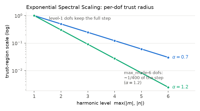
The ESS trust-region weight per harmonic level (\(\alpha = 0.7\) as in the bundled examples, \(\alpha = 1.2\) the ess_alpha default). At \(\alpha = 1.2\) a max_mode-6 dof moves ~400x more cautiously than a max_mode-1 dof.

Measured on a 36-core CPU from a near-circular torus seed (single call, all harmonics released at once; scripts examples/optimization/QA_optimization_ess.py and QI_optimization_ess.py):

class	nfp	residual	seed	achieved	max_mode	dofs	wall
QA	2	QS (1, 0)	2.04e-01	7.2e-06	5	120	14.5 min
QI	1	omnigenity	4.52e-01	1.81e-02 (25x)	6	168	17.3 min

The staged ladder remains available (max_mode=(1, ..., 5)) and reaches comparable precision — QA at QS 3.7e-7 in 25.5 min — but takes ~1.8x longer for the same precision class. Both patterns ship as side-by-side example scripts so the two patterns can be compared directly.

Gradients (vmex.core.implicit)

Derivatives through the equilibrium use implicit differentiation of the converged fixed point: the solve is wrapped in jax.custom_vjp; the forward pass runs the fast (opaque) host solver, and the backward pass solves the adjoint linear system matrix-free with preconditioned GMRES — O(1) memory in the iteration count, no unrolling, no finite-difference step-size to tune. Coarse multigrid stages are just an initializer and are stop-gradient by construction. See the Implicit differentiation section of Algorithms for the formulation and cost analysis.

import jax
from vmex.core import implicit
from vmex.core.input import VmecInput

inp = VmecInput.from_file("input.solovev")
p0 = implicit.params_from_input(inp)

sol = implicit.run(inp, p0)                        # ImplicitSolution pytree
grad = jax.grad(lambda p: implicit.run(inp, p).wb)(p0)   # adjoint gradient

run() is the differentiable member of the entry-point family (see Choosing an entry point in Quickstart; the non-differentiable Python default is solve_equilibrium()). Besides the scalar outputs, the returned solution carries the internally built evaluation context as sol.runtime (a non-pytree convenience attribute), so custom objectives can evaluate further (state, runtime) targets — opt.mean_iota(sol.state, sol.runtime) — without rebuilding the runtime per evaluation.

Gradient accuracy is validated in CI against central finite differences for fixed-boundary degrees of freedom — boundary Fourier coefficients, phiedge, and profile parameters (pres_scale) — on a 2D (solovev) and a 3D (li383) case, with agreement at the 1e-6 relative level (2D) and at the finite-difference noise floor (3D) (tests/test_implicit_grad.py). For solver-sensitive metrics (iota, mirror ratio, magnetic well, the QI residual) a naive re-solving finite difference is not a valid reference — it perturbs the solver’s discrete convergence path, not just the fixed point — and the frozen-path FD (frozen_path_directional_fd()) must be used instead; see Gradient checking: solver-sensitive metrics and the frozen path in Algorithms.

Implicit gradients are not merely faster than finite differences here — on the flagship campaigns they are necessary: the exact-axisymmetric seed is a saddle of the QS residual where finite differences stall, and on the QP class the implicit path selects a better basin.

The gradient stack: what makes a Jacobian cheap

A trust-region iteration spends its time in two places: the Jacobian (one linear solve per dof) and the trial solves (one equilibrium per proposed boundary). The R25 work attacked both, and all of it is on by default:

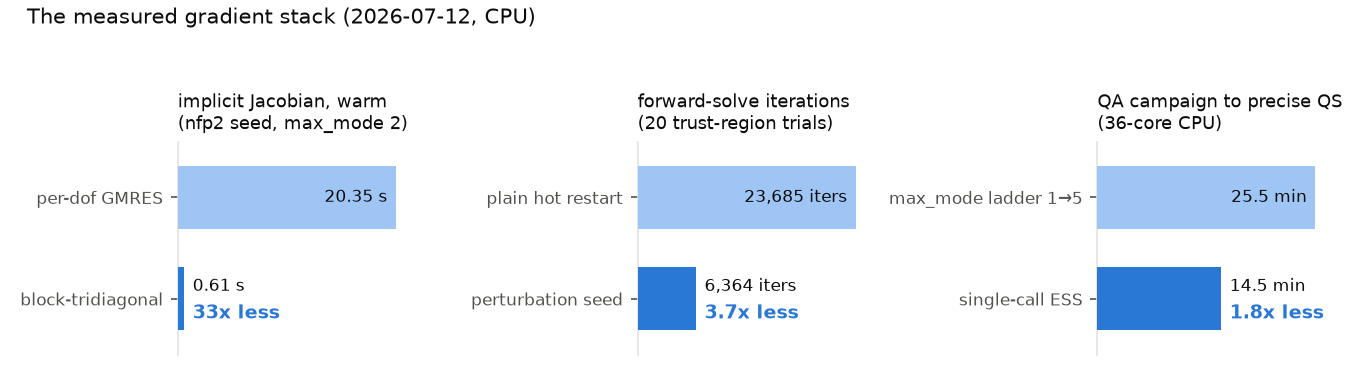
Measured on the nfp2 minimal-seed deck (Jacobian phase and trial iterations) and the full QA campaign (right); 2026-07-12, CPU. Reproduce the campaign numbers with the two examples/optimization/QA_optimization*.py scripts.

• Block-tridiagonal Jacobian factorization (jac_solver="block", default). The raw force Jacobian dF/dz is exactly block-tridiagonal in radius (nearest-neighbor coupling; verified to 1e-14), so ns dense (3mn, 3mn) blocks are assembled with 3-colored jax.jvp probes — a cost independent of the dof count — factored once (solvax.block_thomas), and back-substituted for every dof right-hand side. A short warm-started GMRES corrector certifies each column to the same adjoint_tol as the old path. Measured: the warm Jacobian phase drops 20.35 s to 0.61 s (33x); jac_solver="gmres" (one preconditioned GMRES per dof) remains as a fallback.

• Converged-state memo. scipy’s trust-region drivers call jac(x) at exactly the x that fun(x) just converged; a one-entry params-keyed memo removes that redundant solve per accepted iterate, and the final diagnostic result.equilibrium hot-seeds from the last trial state instead of re-solving cold.

• Perturbation warm start (warm_start="perturbation", default). Each trial solve is seeded with the DESC-style first-order prediction \(z_{\mathrm{ref}} + \sum_j (dx)_j\, dz_j\) — the per-dof state responses \(dz_j\) are exactly the columns the Jacobian already computed, so the linearization is stashed for free at each jac(x) call. Measured: total forward-solve iterations drop 3.7x (23,685 to 6,364 over 20 trials), and the predicted seed rescued a trial whose plain hot restart hit a Jacobian-sign failure. "state" (plain hot restart) and None are the fallbacks; all three converge to identical fixed points.

• Memory stays bounded by column chunking (jac_chunk_size="auto", the same knob DESC exposes): peak Jacobian memory is m0 + m1*chunk instead of scaling with the dof count, and the chunked columns are identical to float64 round-off.

• Krylov recycling (recycle=True) carries a GCROT deflation space across the per-dof solves. It is off by default for a measured reason: solvax v0.1’s FIFO recycle space slows warm-started columns (1.7–3.4x more iterations on the benchmark operator). The plumbing is exact and ready for a harmonic-Ritz GCRO-DR upgrade in SOLVAX; benchmark per-column iteration counts before enabling it.

The end-to-end effect on the profiled production opt_step and the CPU versus GPU placement question are quantified in Performance and validation.

Free-boundary gradients (virtual casing)

Free boundary is differentiable through a different route (vmex.core.freeboundary_diff): rather than differentiating the NESTOR vacuum solve, the plasma-boundary contribution to the vacuum field is computed by virtual casing, which is a smooth function of the coil / extcur parameters and the plasma surface. Coil-parameter derivatives of free-boundary outputs are obtained end-to-end this way and are finite-difference-validated. (The two scopes are complementary: the fixed-boundary implicit adjoint is validated to ~1e-6 relative; the free-boundary virtual-casing path is FD-validated.) See the Differentiable free boundary section of Algorithms.

True single-stage (plasma boundary and coils at once)

The virtual-casing residual is differentiable not only in the coils but also in the plasma boundary: surface_field_data_from_state() rebuilds the virtual-casing surface field traceably straight from a live equilibrium state (bit-exact against the wout path), so a single jax.value_and_grad of a combined objective

J(boundary, extcur) = w_bn * <(B_ext . n)^2>        # coil<->plasma consistency
                    + w_phys * physics(boundary)     # e.g. QS / iota / well

threads through the implicit adjoint (boundary dofs) and virtual casing (coil dofs) simultaneously — the coil residual is evaluated on the boundary the plasma solve just produced, and that coupling is differentiated too. Both blocks are finite-difference validated (coil dofs to ~1e-10; boundary dofs to the FD floor of the re-solved equilibrium).

Making virtual casing differentiable in the boundary needs its adaptive quadrature/patch precision frozen to static values: plan_vc_precision() selects it once from the starting (concrete) boundary and returns a PrecisionPlan to pass back via precision= (the auto-selection otherwise concretizes traced surface values). examples/single_stage_simultaneous_opt.py runs the full loop: from the bundled CTH-like free-boundary equilibrium it reshapes the boundary to move the edge rotational transform while re-tuning the coils to keep <(B.n)^2> small — one exact gradient over both dof families. examples/single_stage_essos_coils_opt.py is the coil-agnostic variant of the same loop, driving the coil half straight from an ESSOS essos.coils.Coils Biot–Savart callable (no mgrid file), and examples/single_stage_free_boundary_opt.py is the coil-only half in isolation — perturb the confining coil currents of the bundled CTH-like case and recover them by minimizing <(B.n)^2> with the exact virtual-casing gradient (finite-difference-validated to ~1e-9).

Worked results

From a near-circular torus seed, jac="implicit" with ESS reaches precise quasisymmetry and strong quasi-isodynamicity (measured on an office CPU): QA (nfp 2) QS 7.2e-6 in one 14.5-minute call (the staged ladder reaches 3.7e-7 in 25.5 min), QH (nfp 4) QS 5.83e-5, QP (nfp 2) QS 9.4e-2 in the single-call budget (the hardest class — basin-limited; the shipped deck reaches 3.3e-2 after an extended ladder plus warm-start refinement), and QI (nfp 1) omnigenity residual 1.81e-2, 25x below the seed, in one 17.3-minute call. The complete scripts are in examples/optimization/ (QA/QH/QP/QI, each with an _ess single-call variant where measured).

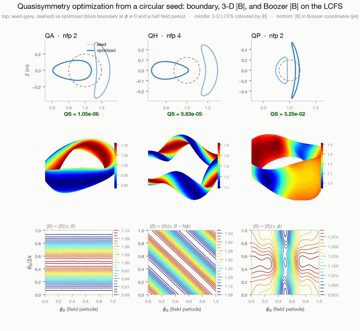
Quasisymmetry (QA/QH/QP): seed (grey) vs optimized (blue) boundary cross sections (top), the optimized LCFS in 3-D coloured by |B| (middle), and |B| in Boozer coordinates on the LCFS (jet line contours, bottom), whose contour geometry reads off the symmetry family. The label is the QS residual measured on the plotted equilibrium. Reproduce with benchmarks/make_readme_figures.py --only optimization from the decks in benchmarks/opt_decks/.

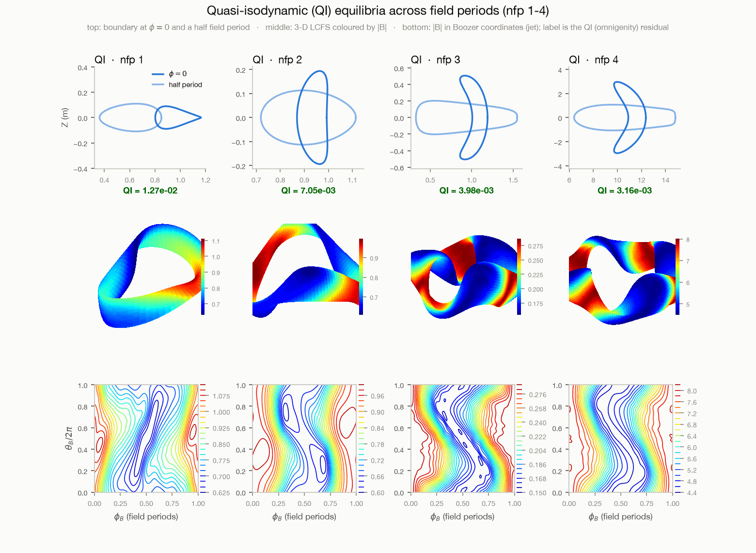
Quasi-isodynamic (QI) equilibria at nfp 1/2/3/4 (bundled decks in examples/data/): boundary cross sections, 3-D |B| geometry, and |B| in Boozer coordinates on the LCFS (jet). The label is the QI (omnigenity) residual, not QS. Reproduce with benchmarks/make_readme_figures.py --only qi.