Mirror geometry

vmex.mirror contains two spline-native scalar-pressure equilibrium models. Open mirrors use coordinates (s, theta, xi) with a nonperiodic axial coordinate and fixed-flux end cuts; they are not reinterpreted as thin periodic tori. Closed stellarator-mirror hybrids use a periodic longitudinal B-spline around two exactly straight mirror legs and two curved stellarator returns. Axisymmetric and rotating-ellipse fixed-boundary open lanes are supported, as is axisymmetric free boundary through 10% requested beta. The periodic hybrid has a complete fixed-boundary solve and example. Its circular-section lane is supported: with the leg-return junction frozen as a design parameter, its independent strong-force residual converges monotonically under same-geometry refinement. The rotating-elliptical-section hybrid remains the single research candidate. section_turns now turns the ellipse continuously around the closed circuit – a genuine rotating-ellipse section – which raises the transform from the return-only iota=0.085 to iota=0.141 at s=0.75, but the separately scoped near-axis representation defect in the rotating section persists at the higher rotation, so it is not promoted.

Quickstart

The easy entry point solves an axisymmetric open mirror from a single LCFS radius, picking a default boundary and profiles for the requested resolution:

from vmex.mirror import MirrorConfig, MirrorResolution, solve_fixed_boundary_from_radius

config = MirrorConfig(resolution=MirrorResolution(ns=7, mpol=4, nxi=17))
result = solve_fixed_boundary_from_radius(0.3, config)

MirrorResolution takes ns (radial surfaces), mpol (largest represented poloidal Fourier mode), and nxi (axial nodes); the returned SplineMirrorSolveResult carries the converged coefficients and the variational, weak, and pointwise-force residuals.

Three runnable examples ship with the package and need no command-line arguments:

python examples/mirror_fixed_boundary_nonaxisymmetric.py   # rotating-ellipse fixed boundary
python examples/mirror_free_boundary_beta_scan.py          # axisymmetric free-boundary beta scan
python examples/stellarator_mirror_hybrid.py               # periodic B-spline racetrack hybrid
python examples/qi_mirror_hybrid_fourier_vs_bspline.py     # QI-mirror hybrid: Fourier vs B-spline

Open-mirror solves write mirror-native mout_*.nc files, which plot with

vmex --plot mout_*.nc

Open topology and end cuts

The open coordinates are \((s,\theta,\xi)\in[0,1]\times[0,2\pi)\times[-1,1]\). The lateral surface \(s=1\) is the plasma-vacuum interface. The planes \(\xi=\pm1\) are prescribed computational cuts through the flux tube; magnetic flux passes through them, so they are neither material interfaces nor B.n=0 boundaries. The divergence-free representation is

\[\sqrt{g}B^\theta = I'(s)-\partial_\xi\lambda, \qquad \sqrt{g}B^\xi = \Psi'(s)+\partial_\theta\lambda,\]

with \(B^s=0\) and a zero-surface-mean gauge for \(\lambda\). All theta samples at the magnetic axis denote one physical point. Writing \(q_0=\lim_{s\to0}r\,\partial_s r\), single-valued axial field requires

\[\partial_\theta\lambda(0,\theta,\xi) = \Psi'(0)\left[\frac{q_0(\theta,\xi)}{\langle q_0\rangle_\theta}-1\right].\]

The solver eliminates the axis stream function with this condition and includes its geometry dependence in variational and implicit derivatives. Axis |B| nonuniformity is stored as a separate axis-uniformity diagnostic.

An unbounded exterior Green solve requires a geometrically closed integration surface, so disks temporarily close the two cuts. Their Neumann data continue the nonzero plasma and applied-field through-flux across each cut. The disks do not close the plasma or acquire an interface pressure-balance equation. Tangency and total-pressure continuity are enforced only on the lateral LCFS. The complete nested radial profile at each cut is prescribed by the initial state and remains fixed during primal and implicit solves. A state built only from the LCFS uses radially self-similar cuts. For a finite-radius supplied field, callers should instead initialize nested cut surfaces from its enclosed flux; otherwise the incompatible cut data appear as a localized strong-force error even when the variational residual is small.

Resolution contract

MirrorResolution(ns=..., mpol=..., nxi=...) has one angular-resolution input: mpol is the largest represented Fourier mode. The plasma collocation size is the read-only value ntheta = 2*mpol + 1; therefore mpol=0 has one theta node and mpol=4 has nine. Users cannot request an inconsistent node/mode pair or accidentally introduce a Nyquist mode. Exterior angular quadrature remains an independent argument because it integrates the vacuum boundary rather than defining plasma unknowns.

Radial location map

The radial mesh follows the VMEC staggering convention, adapted to the two-point Gauss energy rule:

• geometry and stream-function unknowns are stored on full surfaces \(s_i\);

• metric terms, \(\sqrt{g}B^\theta\), \(\sqrt{g}B^\xi\), and magnetic energy are evaluated at two Gauss points inside each radial cell;

• Gauss averages define cell-centered covariant \(B_\theta\), \(B_\xi\), Jacobian, and pressure at \(s_{i+1/2}\);

• current and J x B - grad(p) are reconstructed on interior full surfaces;

• the magnetic axis, fixed LCFS, and open end cuts are reported separately from the unconstrained physical-volume norm.

For open mirrors, bulk and radial-axis diagnostics use the central 80% of the axial coordinate. end_collar uses the outer 20% nearest the two fixed cuts. The all-volume norm retains both regions.

Strong-force gate normalization

The pointwise residual |J x B - grad(p)| is a force density and needs a reference force scale to become a dimensionless gate. The primary normalization divides by \(B^2/(\mu_0 a)\), where the minor radius a is the flux-equivalent LCFS radius: the midplane cross-section for open mirrors and the circuit-averaged section for closed hybrids (vmex.mirror.forces.effective_minor_radius(); a caller may also pass minor_radius explicitly). Transverse pressure balance acts on the minor-radius scale, so \(B^2/(\mu_0 a)\) is the magnitude of the competing equilibrium forces, and every lane has one structural a. The earlier normalization used the device length L (cap-to-cap extent for open mirrors, axis arc length for the closed racetrack). That number is linear in an arbitrary length: open lanes have L/a near 17–20 while the closed racetrack has L/a near 67, so one identical solved hybrid state reads 0.205 arc-normalized but 0.0030 minor-radius-normalized, even though its absolute force density is lower than that of the passing medium rotating ellipse. The device-length number therefore remains available only as the secondary device_normalized_rms diagnostic, and the recorded benchmarks/mirror_*.json files intentionally keep quoting it: they document the historical evidence and are not rewritten under the new normalization.

Gate evaluation reports zones rather than a single folded number: vmex.mirror.forces.force_gate_zones() returns the all-volume, bulk, end-collar, and near-axis/first-row norms (all minor-radius-normalized) together with the legacy device-length total, so constrained-data regions – the frozen end cuts and the regularized axis – are visible next to the unconstrained bulk. Promotion additionally requires refinement evidence: vmex.mirror.forces.refinement_convergence() reports per-step ratios and monotonicity for residuals from two or more resolutions, and vmex.mirror.forces.passes_promotion_gate() combines the absolute gate on the finest rung with that monotone-decrease requirement.

Re-measured gate numbers for the shipped cases, evaluated on the identical solved states under both normalizations (device-length L-normalized values match the recorded evidence bit-for-bit):

Case	device norm	minor norm	bulk	end collar	axis row
Rotating ellipse (ns,mpol,nxi,elements) = (5,4,13,5)	0.0667	0.00400	0.00231	0.00683	0.00343
Rotating ellipse (7,6,17,6), the supported lane	0.0267	0.00160	0.00073	0.00274	0.00196
Rotating ellipse (9,8,21,8)	0.0142	0.00085	0.00026	0.00156	0.00060
SFLM (7,6,17,6), paraxial benchmark	0.335	0.0168	0.00259	0.0350	0.00863
SFLM (9,8,21,8), paraxial benchmark refined	0.177	0.00883	0.00140	0.0169	0.00442
Hybrid circular section, frozen junction, ns=5, 16 controls	0.204	0.00304	0.00304	(none)	0.00261
Hybrid circular section, frozen junction, ns=5, 32 controls	0.176	0.00261	0.00261	(none)	0.00196
Hybrid circular section, frozen junction, ns=5, 64 controls	0.118	0.00175	0.00175	(none)	0.00084
Free boundary (ns,nxi,elements,panels) = (5,7,4,8), beta 0	0.0421	0.00665	0.00610	0.00718	0.00431
Free boundary (5,7,4,8), beta 10%	0.0269	0.00430	0.00490	0.00361	0.00588

The rotating-ellipse ladder stays monotone under the new normalization (per-step ratios 2.50 and 1.88), and the frozen-junction circular-section hybrid ladder is likewise monotone (minor-radius bulk 0.00304 -> 0.00261 -> 0.00175, device-normalized all-volume 0.204 -> 0.176 -> 0.118): with the junction geometry held fixed, exact refinement of the solve basis drives the force down instead of plateauing. Its minor-radius number sits between the coarse and medium open rungs instead of appearing an order of magnitude worse: the apparent cross-lane gap was the L/a disparity, not a larger force error. The straight field-line mirror (SFLM) is a paraxial-accuracy benchmark rather than a failed case: its unconstrained bulk force is clean (0.00259 minor-normalized, below the 0.05 gate) and converges under refinement – the (7,6,17,6) -> (9,8,21,8) step halves it, 0.00259 -> 0.00140 (ratio 1.85), and the all-volume and end-collar norms fall in step (0.0168 -> 0.00883 and 0.0350 -> 0.0169). The elevated end collar is the expected boundary layer where the analytic Agren–Savenko cut profile, an equilibrium only to order (a/c)^2, is frozen at the two end cuts; it converges rather than plateaus.

In particular, radial curl and pressure terms use conservative cell differences,

\[\sqrt{g}J^\theta_i = \frac{1}{\mu_0} \left[\partial_\xi B_{s,i} - \frac{B_{\xi,i+1/2}-B_{\xi,i-1/2}}{\Delta s}\right],\]

\[\sqrt{g}J^\xi_i = \frac{1}{\mu_0} \left[\frac{B_{\theta,i+1/2}-B_{\theta,i-1/2}}{\Delta s} - \partial_\theta B_{s,i}\right], \qquad p'_i = \frac{p_{i+1/2}-p_{i-1/2}}{\Delta s}.\]

Contravariant field on a full surface is reconstructed by averaging flux density and Jacobian separately, rather than averaging their ratio. This is the same placement used by VMEC2000 jxbforce and avoids differentiating an unrelated full-mesh reconstruction of the energy field.

Current capability and limits

The package currently includes:

• supported axisymmetric and nonaxisymmetric fixed-boundary finite-current solves,

• an isotropic VMEC-style conserved-mass pressure energy with independent weak and pointwise force diagnostics,

• a free-space boundary-integral vacuum model with an xyz -> B field callable or the shared ESSOS/MAKEGRID-compatible MgridField; coil geometry and Biot-Savart evaluation remain in ESSOS,

• coupled axisymmetric free-boundary beta continuation with compressed restart files,

• a closed-surface Neumann solve on the lateral LCFS and both end disks,

• component-wise nonlinear convergence checks at a requested ftol=1e-12.

• a periodic B-spline racetrack with two straight mirror legs, a continuously rotating elliptical section, a fixed-boundary solve, and closed field-line tracing.

With the compact-coil configuration (0.5 m loops, vacuum B(0) = 0.0836 T, mirror ratio 4.58), a requested 50% beta continuation grows the central radius by 7.5% and lowers the on-axis field by 22.3% from vacuum, exercising the finite-beta coupling end to end. The axisymmetric free-boundary path is supported through 50% requested beta: a size-scaled Krylov span in the Newton-GMRES polish (restart = max(24, min(problem.size, ...))) clears the fine-grid restart starvation that previously stalled the polish short of ftol, and a fine grid (ns=13, nxi=25, elements=13, exterior_ntheta=24) converges every beta point from 0 through 50% (≤ 44 Newton-GMRES iterations, variational residual ≤ 8.5e-15) with bulk minor-radius force rising from 1.21e-4 (beta 0) to 2.41e-3 (beta 50%) — far under the 0.05 gate (see the fine_grid_promotion.fine_grid_50 block in benchmarks/mirror_free_boundary_axisymmetric.json). The nonaxisymmetric free-boundary path is deferred because its point observables were not monotone under spatial refinement.

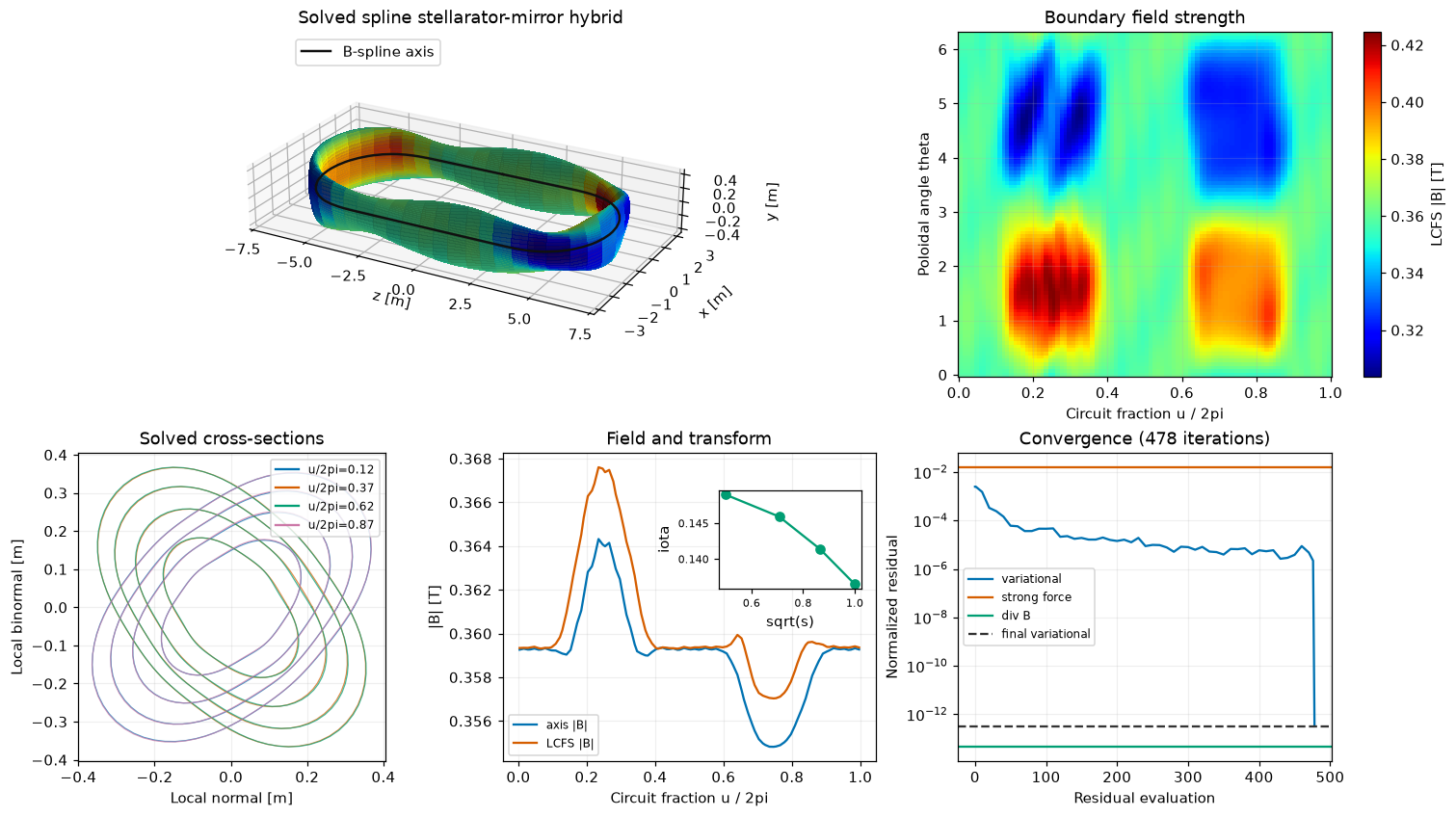
Periodic stellarator-mirror hybrid

The implemented target follows the topology proposed for stellarators linking axisymmetric mirrors (SLAM): two long straight mirror legs are joined by two curved stellarator sections. The same topology appears in the APS linked-mirror abstract. It is related to, but geometrically distinct from, the warm-stellarator/rectilinear-mirror fusion–fission hybrid proposed by Moiseenko et al.. The implementation uses de Boor’s local cubic B-spline construction and Bishop’s rotation-minimizing frame. The present code addresses only ideal-MHD nested-surface geometry and a scalar-pressure equilibrium. It does not model fusion–fission blankets, minority fast ions, end losses, or kinetic stability.

Let \(u\in[0,2\pi)\) parameterize the closed circuit. The coordinate map is

\[\boldsymbol x(s,\theta,u) = \boldsymbol c(u) + \sqrt{s}\,a(s,\theta,u) [\cos\theta\,\boldsymbol n(u)+\sin\theta\,\boldsymbol b(u)].\]

CubicBSplineBasis.periodic_uniform represents \(\boldsymbol c\). Control points are divided between straight leg, return, opposite straight leg, and second return. A cubic spline has local support, so every central span whose four active controls are collinear is exactly straight; increasing the number of controls lengthens the exact straight region rather than merely improving a global Fourier fit. evaluate_closed_spline_axis transports a Bishop rotation-minimizing frame \((\boldsymbol n,\boldsymbol b)\) around the curve and distributes its residual holonomy over the period. This frame is well defined where the straight-leg curvature is exactly zero, unlike the Frenet frame.

The LCFS is an ellipse written as a polar radius,

\[a(1,\theta,u) = \frac{A B}{\sqrt{[B\cos(\theta-\alpha(u))]^2 +[A\sin(\theta-\alpha(u))]^2}}.\]

The section angle is \(\alpha(u)=\alpha_{\mathrm{ret}}(u)+N\,u\). The return term \(\alpha_{\mathrm{ret}}\) is constant on each straight leg and changes smoothly by 90 degrees through each return, so on its own it returns the ellipse to its original orientation once per circuit. The section_turns integer \(N\) superposes a genuine rotating ellipse: the major axis turns continuously by \(N\) full \(2\pi\) turns per circuit. Because the polar radius is \(2\pi\)-periodic in \(\theta-\alpha\) and \(N\) is an integer, the section closes on itself exactly (verified by the m=2 harmonic winding by \(4\pi N\)), and the straight-leg axis stays exactly straight while the ellipse it carries keeps rotating. The radial surfaces and stream function use the same periodic longitudinal basis. The divergence-free field is the open expression with \(\xi\) replaced by \(u\); periodicity removes end cuts, and all longitudinal coefficients are active. A finite \(I'(s)\) gives visible pitch and nonzero rotational transform; at the device aspect ratio \(L/a\approx 67\) the rotating ellipse adds negligible transform on its own (with \(I'(s)=0\) the traced \(\iota\) stays below \(10^{-3}\) for every section_turns), so it acts by amplifying the current-driven transform rather than by a standalone geometric one.

build_stellarator_mirror_hybrid constructs the discretization, closed axis, LCFS, and a vacuum-field initial stream function. The ordinary solve_fixed_boundary then uses the same energy, host globalization, matrix-free Hessian actions, and separable preconditioner as open mirrors. trace_closed_field_line integrates \(d\theta/du=B^\theta/B^u\) with periodic RK4 steps. The parser-free root example is:

python examples/stellarator_mirror_hybrid.py

The leg-return junction – where an exactly straight leg (zero curvature) meets a circular return (curvature \(1/R\)) – is rounded across the cubic spline’s local support. Building the axis directly in a finer solve basis narrows that rounding and sharpens the junction curvature overshoot as fast as refinement helps, so the as-built geometry family does not converge: the circular section reads 0.184 device-normalized at 32 controls and 0.218 at 64. build_stellarator_mirror_hybrid(axis_coefficient_count=...) freezes the junction as an explicit design parameter of the closed B-spline axis family. The racetrack axis and rotating section are constructed at that base control count and then exactly refined (refine_periodic_uniform, dyadic and curve-preserving to roundoff) to the solve coefficient_count, so the junction-transition width is held fixed while the equilibrium resolution increases. The default axis_coefficient_count=None keeps the legacy behaviour of building the geometry in the solve basis.

With the junction frozen at 16 controls, the circular-section hybrid converges monotonically under exact 16/32/64 solve refinement: device-normalized all-volume force 0.204 -> 0.176 -> 0.118 (reproducing the audit ladder) and minor-radius bulk force 0.00304 -> 0.00261 -> 0.00175 (per-step ratios 1.16 and 1.49), every rung below the 0.05 gate with variational residual below 3.2e-13 and normalized div(B) below 1e-13. This passes the promotion criterion (absolute gate on the finest rung and monotone refinement), so the circular-section hybrid is a supported lane. Every hybrid residual in this section is quoted device- (arc-length-) normalized where noted (the legacy normalization recorded in benchmarks/mirror_hybrid_fixed_boundary.json); the racetrack arc length is about 67 minor radii, so the device numbers are roughly 67 times the minor-radius numbers.

The rotating-elliptical-section hybrid remains the single research candidate, now driven by the genuine toroidal rotation section_turns. Its shipped ns=5, mpol=4, 32-control case (semi_major=0.45, semi_minor=0.25, section_turns=2) reaches variational residual 3.19e-13 and normalized div(B)=4.55e-14 with axis closure 8.88e-16, and the solved finite-current state gives iota=0.141 at s=0.75 – roughly 1.7 times the return-only iota=0.085 at the same imposed current. The transform is current-driven and amplified by the rotating geometry: with I'(s)=0 the traced transform stays below 10^{-3} for every section_turns, so at L/a near 67 the rotating ellipse adds no standalone geometric transform and instead reshapes the metric so the same current winds field lines faster.

Under the junction-freeze contract the toroidally rotating hybrid converges at every rung, but the near-axis defect persists. With the junction frozen at 16 controls and the section built at that base count, exact 16/32/64 refinement (ns=5, mpol=6, section_turns=2) drives the minor-radius bulk force 0.0445 -> 0.0056 -> 0.0046 – monotone, every rung below the 0.05 gate, so the operational promotion gate passes – with each rung at variational residual below 3.6e-13 and normalized div(B) below 1e-13. The device- (arc-length-) normalized strong force, however, plateaus 4.07 -> 0.51 -> 0.42 (per-step ratios 7.97 and 1.21): it does not head toward zero like the promoted circular lane (0.204 -> 0.176 -> 0.118), and its ~0.42 floor is even higher than the return-only ~0.33. That plateau is the same separately scoped near-axis representation defect in the rotating section, made no better by the faster rotation, so the toroidally rotating hybrid is kept a research candidate; finite-beta continuation and rotating-section sensitivity claims are deferred until it is resolved.

A sensitivity study on the return-only baseline localizes the rotating-section residual to the racetrack geometry rather than to pressure or imposed current. At the 32-control resolution, removing current changes the return-only strong force only from 0.430 to 0.424; replacing the rotating ellipse by a circular section gives 0.158 and a fixed ellipse 0.164, while the circular-axis/circular-section limit gives 0.0083. The periodic derivative algorithm is validated separately on the closed circular limit below.

Source ownership is compact: periodic basis/refinement is in basis.py; axis, Bishop frame, and embedding are in geometry.py; coefficient packing, initialization, solve dispatch, and tracing are in splines.py; the shared energy and force diagnostics are in forces.py; and the reviewed figure is produced by output.plot_stellarator_mirror_hybrid.

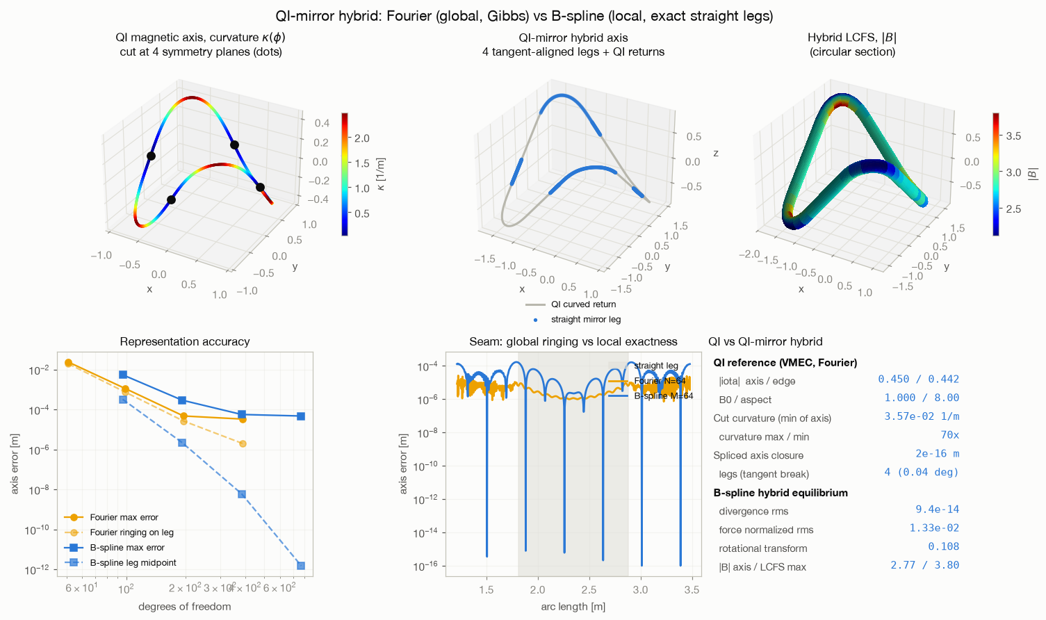
QI-mirror hybrid: Fourier vs B-spline

A quasi-isodynamic (QI) stellarator has poloidally closed |B| contours and near-straight magnetic-axis segments at its field-period-symmetric planes, so the QI axis is the natural place to cut and insert a straight mirror cell. examples/qi_mirror_hybrid_fourier_vs_bspline.py makes that construction concrete and compares the two ways of representing the resulting axis.

Cut locations. The example solves input.nfp2_QI with the VMEC (Fourier) core, reads the magnetic axis \(\mathbf{r}(\phi)\) from the axis Fourier arrays, and computes the 3-D curvature \(\kappa = \lVert \mathbf{r}' \times \mathbf{r}'' \rVert / \lVert \mathbf{r}' \rVert^{3}\) spectrally over the torus. For this nfp=2 QI the curvature spans 70x. An nfp=2 QI axis is near-straight at two planes per field period, so the curvature has four minima: \(\kappa \approx 0.036\) \(\mathrm{m}^{-1}\) at \(\phi = 0, \pi\) and \(\approx 0.088\) \(\mathrm{m}^{-1}\) at \(\phi = \pi/2, 3\pi/2\) (the four stellarator-symmetry planes, where the axis crosses the midplane), and maxima \(\approx 2.5\) \(\mathrm{m}^{-1}\) at the bean tips. All four low-curvature planes are cut, so the inserted legs are stellarator symmetric.

Cut-and-splice. splice_straight_legs cuts the closed axis at the four minima and inserts an exactly-straight leg at each along the local axis tangent, so every leg continues the axis in its own direction (not a shared transverse direction). The per-cut leg lengths are chosen so the inserted displacements cancel – the loop closes to rounding (closure ~ 1e-16) – which splits the legs into two symmetry classes (the two symmetry-plane types, here 1.31 m and 1.07 m). One stellarator-symmetric half, between the two symmetry-fixed planes, is built and reflected 180 degrees about the x axis, so the four-legged racetrack is stellarator symmetric to rounding. Each leg is tangent to the axis at its cut, so the leg/return junction is tangent-continuous (residual break ~0.04 deg, versus a real corner): the seam is now a curvature break – the exactly-zero-curvature leg meeting the finite-curvature return – which is what separates the two representations.

Representation accuracy. The same closed hybrid axis is fitted with a truncated Fourier series (global, VMEC-native) and a periodic cubic B-spline (local, the vmex.mirror lane). On the straight mirror leg:

basis	degrees of freedom	deviation on the straight leg
Fourier, \(N=8\)	51	2.0e-2 (ringing)
Fourier, \(N=32\)	195	2.7e-5 (ringing)
Fourier, \(N=64\)	387	2.0e-6 (ringing, floor)
B-spline, \(M=64\)	192	2.2e-6 (leg midpoint)
B-spline, \(M=128\)	384	6.0e-9 (leg midpoint)
B-spline, \(M=256\)	768	1.5e-12 (leg midpoint)

The B-spline reproduces the straight cell to machine precision once each leg is backed by enough collinear controls (its error is confined to a fixed few knot-spacings around the junction, the signature of local support), while the global Fourier series rings across the whole leg and floors near 2e-6. The tangent-continuous seam lets the Fourier ringing decay faster than the old sharp-corner case, but only the local basis reproduces the exactly-straight cell to machine precision. The maximum error of both bases is instead set by the leg/return curvature break (a cubic B-spline is \(C^2\) and also rounds a curvature step), so this is an honest, shared limit, not a B-spline advantage. The comparison is the point: the local basis wins precisely on the exactly-straight mirror cell.

Equilibrium. build_qi_mirror_hybrid fits the spliced axis into the closed solve basis, wraps it in a constant circular section (rotation-invariant, so the large frame holonomy of a fully 3-D axis does not enter the boundary), and returns a StellaratorMirrorSetup that feeds solve_fixed_boundary like the analytic racetrack. The solved hybrid is divergence-free to 9.4e-14 with iota = 0.11 and mirror ratio 1.8; its normalized strong-force residual is 1.3e-2 (the smooth analytic racetrack, with circular returns, converges to 2.6e-3 by contrast – the QI returns’ finite curvature and the four curvature-break seams still load the force). This B-spline equilibrium is a scalar-pressure spline model whose transform comes from a weak axial current: it demonstrates the geometry and the exactly-straight mirror cell, not a reproduction of the QI rotational transform (|iota| ~ 0.45).

Fourier-lane limitation. A literal VMEC re-solve of a straight-axis QI-mirror device is out of scope by construction, not by effort: VMEC’s toroidal coordinate is the cylindrical angle \(\phi\), and a straight axis segment cannot be parameterised by \(\phi\) (its \(R(\phi), Z(\phi)\) are degenerate). This is exactly why the closed-axis, arc-length-parameterised B-spline lane exists. The VMEC solve therefore serves as the QI reference (axis, iota, |B|, B_0), and the Fourier side of the comparison is the axis-representation accuracy above.

Plotting and output scope

Open straight-axis examples write mirror-native mout_*.nc files and render horizontal 3D, coil, cap-to-cap field-line, |B|, pressure, cross-section, and residual figures. The same figures can be regenerated with vmec --plot mout_*.nc. The data include geometry, the stream function, Cartesian magnetic field, isotropic pressure, interface residuals, solver history, normalized variational, staggered-weak, and pointwise-force residuals, normalized div(B), and optional coil curves. The variational residual defines ftol. The staggered weak residual independently assembles the first variation on the energy quadrature and is checked on the same constrained solver variables. The pointwise force reconstructs J x B - grad(p) on the full mesh. It does not define nonlinear ftol, but its magnitude and refinement are independent diagnostics. Its total, near-axis, first-radial-row, bulk, and end-collar norms are reported separately, all under the primary minor-radius normalization; the legacy device-length total remains available as device_normalized_rms. div(B) checks the field representation. Open mirror data are never encoded as a toroidal WOUT file. The closed hybrid currently writes a reviewed PNG and JSON summary directly from the solved objects; a periodic MOUT schema is deliberately not inferred from the open end-cut schema.

The saved |B| array is reconstructed from the same radial Gauss cells used by the magnetic-energy functional. Cartesian field samples remain separate for field-line direction. Plots resample the uniformly spaced poloidal data with their resolved Fourier modes, so low-order ellipses are not displayed as polygons.

The compact six-point isotropic data are recorded in benchmarks/mirror_free_boundary_axisymmetric.json: the axisymmetric free-boundary path is supported through 10% beta and retained as labeled validation through 50%. The recorded force values use the legacy device-length normalization (the coarse supported rows re-measured under the minor-radius normalization appear in the gate table above). A refinement matrix over radial, axial, exterior-angular, exterior-order, and combined resolutions gives, at 10%, fine all-volume/core forces 1.44e-2/1.62e-3 with every independent fine force below 2.47e-2. At 25% one independent force reaches 5.70e-2, and at 50% the fine force is 6.69e-2 with a medium-to-fine center-field change of 1.02%. Small variational residuals do not override those independent force values.

Fixed-boundary 3D solver

The fixed-boundary host solver jointly advances geometry and a gauge-free stream function for helical boundaries with finite axial current. Its Newton preconditioner combines radial, Fourier-poloidal, and CGL-axial model stiffness. The eliminated weighted-mean stream-function node is handled by a symmetric lift and projection, so the reduced preconditioner remains positive definite.

The formal full-physics test refines (ns,nxi) through (5,5), (7,7), and (9,9) at mpol=1 and requires component-wise residuals below 1e-12. Radial magnetic energy uses two-point Gauss integration. This is essential: the former midpoint rule admitted an alternating lambda hourglass mode and its published refinement data were rejected. The corrected lambda and pitch profiles are smooth, and a dedicated regression test assigns the alternating mode finite energy.

Two manufactured pointwise-force fixtures isolate the reconstruction from the nonlinear solve. A cylindrical finite-beta state with analytic radial B_z(s) and pressure balance converges at second order when ns doubles. A theta-dependent self-similar tube carrying an exactly uniform Cartesian field gives normalized Lorentz force below 1e-12. These fixtures show that radial differentiation and nonaxisymmetric coordinates work independently; they do not by themselves validate shaped solved states whose pointwise force remains large. The first corrected rotating-ellipse audit also exposed a missing axis condition: the old state varied |B| by 9–20% over theta at s=0 even though those samples are one physical point. That freedom has been removed; the canonical fixed-open records have since been regenerated with the regular axis, while older shaped values remain invalid.

Independent nonaxisymmetric analytic fixtures

vmex.mirror.analytic contains validation data that never call an equilibrium solve. RotatingEllipseParaxial maps a unit circle through a flux-conserving ellipse whose major axis turns by 90 degrees from one end to the other. A compensating field-line-label angle makes the first-order vacuum identity vanish while preserving

\[X_{1c}Y_{1s}-X_{1s}Y_{1c}=\bar B/B_0.\]

It evaluates the Rodriguez-Helander-Goodman Appendix-C Riccati equation and the independent general and magnetic-well-minimum formulas for (B20,B2c,B2s). Tests recover those coefficients from low-radius Fourier samples and verify that the order-r m=1 field strength is zero. This is the coefficient oracle for the native-spline fixed-boundary solve; it is not itself an equilibrium.

StraightFieldLineMirror implements the Agren-Savenko paraxial scalar potential, on-axis field, Clebsch labels, straight nonparallel field lines, and analytic elliptical sections. Its tests verify curl-free field, the expected order-(a/c)^2 solenoidal and field-line truncation errors, axial flux conservation, and

\[B_0(z)=\frac{B_0(0)}{1-z^2/c^2}, \qquad \mathcal E(z)=\frac{1+|z/c|}{1-|z/c|}.\]

Both fixtures require a thin tube and |z|<c. The long-thin ordering treats beta and lambda=(a/L)^2 as simultaneous small parameters; B/B_vac=sqrt(1-beta) is an asymptotic pressure-balance reference, not a finite-beta solution or ellipticity prediction.

Native spline basis status

vmex.mirror.splines.CubicBSplineBasis supplies the longitudinal basis. Open mirrors use clamped knots, exact endpoint values, Gauss-Legendre quadrature on every nonzero span, and exact Boehm knot insertion. Closed hybrids use folded uniform periodic cubic splines and exact dyadic refinement. Evaluation and two derivatives are JAX operations. Tests match SciPy, reproduce cubics, preserve open and periodic curves under refinement, verify partition of unity and C2 closure, and check JVP/VJP actions.

SplineMirrorState and SplineMirrorBoundary store geometry and stream function coefficients rather than sampled values. SplineMirrorDiscretization evaluates them on endpoint-augmented Gauss nodes before calling the shared geometry and energy kernels, and applies side/end constraints plus the lambda gauge in coefficient space. A quadratic flared tube uses 9 coefficients and 26 evaluation nodes versus 41 Chebyshev nodes; volume agrees to roundoff, total energy agrees to 5.0e-13 relative, and an energy directional derivative agrees with finite differences to 1.9e-8 relative.

The public solve_fixed_boundary minimizes the scalar-pressure energy directly in the active spline coefficients. It fixes the side and end coefficients, eliminates the weighted stream-function gauge, and uses the shared host L-BFGS plus residual-Newton policy. The independent staggered first variation is assembled on the quadrature grid and pulled back through the spline evaluation matrix rather than reused from autodiff. The convenience wrapper solve_fixed_boundary_from_radius(radius, config) builds a default axisymmetric boundary of the requested LCFS radius and runs this solve in one call.

For an ns=5 finite-pressure, finite-current flared tube, both paths converge in 59 iterations below ftol=1e-12. Seven spline coefficients replace nine Chebyshev axial nodes and reduce active variables from 45 to 31. Relative differences are 5.1e-7 in energy, 5.9e-6 in volume, and 3.2e-4 in center radius.

Independent solves at (ns,nxi)=(5,9),(7,13),(9,17) pair 7, 9, and 11 spline coefficients with the nodal grids. Energy error decreases 5.12e-7 -> 1.46e-7 -> 5.60e-8, volume error decreases 6.50e-6 -> 2.24e-6 -> 9.85e-7, and sampled radius RMS error decreases 2.40e-4 -> 6.49e-5 -> 2.94e-5. On the finest grid the Cartesian field and |B| differ by 7.02e-4 and 3.05e-4 RMS. Splines use roughly half the active radius variables at all variational and independent weak residuals below 1.3e-15. Compact evidence is in the axisymmetric_refinement section of benchmarks/mirror_fixed_boundary.json.

Open fixed-boundary systems use exact JAX Hessian-vector products and matrix-free Newton at every size. Radius-only systems retain the inexpensive radial/Fourier/axial tensor inverse. Finite-current nonaxisymmetric systems freeze a sparse local Hessian at the start of Newton: columns are evaluated in batches of at most 32, only same-field-channel terms with neighboring radial rows and axial coefficient distance at most four are stored, and all poloidal coupling is retained. Sparse LU is reused for every Newton step; no dense Hessian is stored.

On the 591-variable analytic-seeded SFLM, the frozen local factor reaches true relative residual 9.18e-11 in 660 Krylov iterations where the plain tensor baseline stalls at 7.83e-2 after 2,000, at the same final energy and strong force. Tangent and adjoint systems reuse the traceable separable preconditioner; the host sparse factor remains a primal acceleration and is not differentiated.

On the flared finite-beta case, knot refinement from 5 to 11 coefficients reduces relative energy error against an nxi=17 Chebyshev oracle from 1.09e-6 to 5.14e-8 and volume error from 1.19e-5 to 2.18e-6. Both errors decrease at every refinement and all coefficient solves retain variational and staggered residuals below 9e-15.

Nonaxisymmetric spline evidence

Changing a prescribed spline boundary uses SplineMirrorDiscretization.transfer_boundary. It rescales every nested surface at spline collocation nodes before projection, instead of replacing only the LCFS and risking crossed surfaces. The optimizer also rejects any trial with a changed Jacobian sign, matching the regular VMEC-JAX merit policy.

The old zero-stream continuation produced a nonconvergent strong-force floor. Supplied-field initialization provides the physical stream function and flux, and impose_self_similar_cuts fixes each end section to scaled copies of its LCFS. With these corrected cut semantics, the medium 90-degree rotating ellipse has variational residual 2.11e-16, independent weak residual 2.08e-16, all-volume strong force 2.67e-2 device-normalized (1.60e-3 under the primary minor-radius normalization), and normalized divergence 6.68e-15 at LCFS radius 0.12 m. This is the current supported nonaxisymmetric fixed-boundary case.

initialize_from_cartesian_field now keeps a supplied spline geometry fixed, infers \(\Psi'(s)\) from the surface-averaged axial flux, and obtains the nonzero poloidal stream-function modes from the remaining contravariant field. It accepts either Cartesian field samples or a point callable and performs no coil construction or Biot–Savart integration. The independent Agren–Savenko field is a paraxial-accuracy benchmark: it is an exact equilibrium only to order \((a/c)^2\) (its solenoidal residual is \(O((a/c)^2)\approx 1.6\times10^{-3}\)), so it is gated on its clean unconstrained bulk force and on the refinement convergence of that force, not on a single all-volume number. At (ns,mpol,elements)=(7,6,6) and LCFS radius 0.10 m, the corrected-cut solve reaches variational residual 1.71e-16 and divergence 7.04e-15; its minor-radius-normalized bulk force is 2.59e-3 (well below the 0.05 gate), while the all-volume and end-collar norms are 1.68e-2 and 3.50e-2 (0.335 and 0.701 device-normalized). The end collar is the expected boundary layer where the analytic cut profile, which does not satisfy the discrete equilibrium to machine precision, is held fixed at the two end cuts. Refining once to (9,8,21,8) halves the bulk force to 1.40e-3 (ratio 1.85) and lowers the all-volume and end-collar norms to 8.83e-3 and 1.69e-2, so every zone converges under refinement; it therefore ships as a validated paraxial benchmark, distinct from the supported rotating ellipse, whose section is an exact discrete flux surface.

The parser-free root example runs both fixtures through five coefficient-space continuation stages, solves a standard axisymmetric mirror through solve_fixed_boundary_from_radius, and writes MOUT plus horizontal 3-D, cross-section, |B|, residual, symmetry, and analytic-direction figures:

python examples/mirror_fixed_boundary_nonaxisymmetric.py

The example checks every convergence gate for the rotating ellipse and the axisymmetric mirror, and gates the SFLM benchmark on its clean bulk force (force_gate_zones(...).bulk below the 0.05 gate) while reporting the expected cut collar. Its figures expose variational and reconstructed-force histories and show actual solved nested surfaces and cap-to-cap field lines, not the analytic target alone. 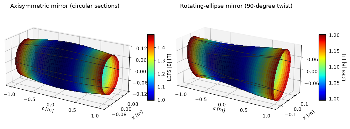The paired 3-D figure below shows the two solved supported lanes side by side, coloured by the local LCFS |B|: the circular-section axisymmetric mirror (mirror ratio 1.5) and the 90-degree rotating ellipse.

Coefficient fixed-boundary gradients

spline_fixed_boundary_adjoint differentiates a scalar diagnostic through the converged coefficient residual. Boundary and periodic-axis spline coefficients, flux, conserved mass, and current remain differentiable. The transpose Hessian action uses exact JAX reverse AD and the nonlinear iteration history is never differentiated or stored. The root example differentiates rotating-ellipse volume with respect to a native boundary coefficient and checks it against two fully reconverged equilibria:

python examples/mirror_fixed_boundary_nonaxisymmetric.py

For the corrected-cut rotating ellipse, the volume adjoint agrees with two fully reconverged centered-difference solves to 5.91e-10 relative and its transpose linear residual is 2.30e-10. An SFLM adjoint is not reported because it is a paraxial-accuracy benchmark rather than a supported equilibrium: its analytic cut profile is fixed input data, not a solved exact discrete flux surface, so a shape derivative through it is not a meaningful optimization sensitivity.

spline_fixed_boundary_tangent solves the complementary forward system F_u du = -F_p dp with exact residual JVPs and the same preconditioner. On a nonaxisymmetric finite-current solve_lambda=True case, both radius and stream-function tangents agree with two fully reconverged centered differences within 2e-4 in relative state norm, with linear residual below 1e-8. This establishes both open-spline derivative directions. On the closed circular limit, periodic boundary and axis controls pass the parameter JVP/VJP transpose identity and an adjoint volume derivative agrees across three fully reconverged centered-difference steps. This validates the closed algorithm for optimization. The supported circular-section racetrack, whose frozen-junction strong-force reconstruction converges under refinement, is a valid sensitivity target; the rotating-elliptical-section racetrack does not yet carry a sensitivity claim while its independent strong-force reconstruction plateaus on the separately scoped near-axis representation defect.

Public fixed-boundary inputs are SplineMirrorBoundary, SplineMirrorState, and SplineMirrorDiscretization; public solve_fixed_boundary returns a SplineMirrorSolveResult. CGL values remain available for quadrature and evaluated-state parity tests, not as a second production state.

Axisymmetric free-boundary implicit gradients

free_boundary_adjoint differentiates the axisymmetric exterior equilibrium with respect to a differentiable external-field callable, axial flux, conserved mass profile, and axial current. The physical fixed point contains the lateral LCFS and plasma-interior radii. The exterior Neumann BIE eliminates vacuum unknowns, so its exact reverse-AD field and shape responses enter the interface-stress rows directly. The transpose solve reuses the separable primal plasma preconditioner and does not assemble a dense Jacobian or retain nonlinear iterations.

The validation uses a differentiable curl-free paraxial mirror field and checks both its strength/axial-curvature controls and a finite-pressure mass direction against fully reconverged equilibria. Pressure changes through the same conserved-mass and solved-volume relation as the primal. End-cut radii and any central-pressure calibration target remain fixed. Coil-design derivatives belong to the ESSOS integration layer; VMEX differentiates only the supplied field object.

The adjoint consumes the same primal coefficient residual, coefficient packing, and block preconditioner. It is supported through the 10% beta ceiling and is checked against fully reconverged field and mass perturbations: the implicit free-boundary derivative matches a reconverged finite difference to 1.1e-10 relative (transpose linear residual 1.4e-9). The nonaxisymmetric free-boundary derivative is deliberately unavailable because local Fourier-mode refinement failed; it will not be presented as a supported gradient.

device=None uses the shared measured device policy. On the office host, the corrected 15x15 case took 35.2 seconds on CPU and 44.2 seconds on one RTX A4000. Energy and force diagnostics agree to numerical precision. Explicit device= arguments and JAX platform environment pins are always honored.

Fixed- and free-boundary derivatives solve the linearized converged coefficient residual and never retain or differentiate the nonlinear iteration history. The mirror CPU path uses SciPy GMRES around exact JAX JVP/VJP actions; no accelerator solver option is exposed because the one-shot derivative API cannot amortize a SOLVAX solver’s first compiled solve.

Beta scan example

From a developer checkout, run:

python examples/mirror_free_boundary_beta_scan.py

The script has editable inputs at its top and no command-line parser. It solves every beta point from 0 through 50% and writes one MOUT per state, a compact JSON summary, restart files, and reviewed figures under results/mirror_free_boundary_beta_scan/. The figures include horizontal z geometry, LCFS displacement, on-axis and LCFS |B|, pressure balance, coils, cap-to-cap field lines, and coupled residual histories, plus one composite summary pairing the solved 3-D states with whole-scan diagnostics. Generated results are ignored by git. Every beta point from 0 through 50% is supported: the fine-grid promotion run above ((13,25,13,24) grid, size-scaled Krylov span, minor-radius force normalization) converges each point below the 0.05 bulk gate. The per-grid figures in the two paragraphs that follow predate that fix and use the legacy device-length force normalization on a coarser exterior grid, so their higher strong-force numbers are a coarser-grid legacy diagnostic, not the operational gate.

The default free-boundary center radius remains 0.25 m. The example’s two ESSOS loops are sized to the plasma: radius 0.5 m at z = +/-1.0 m carrying 3.72e5 A each. This reproduces the central vacuum field B(0) = 0.0836 T of the recorded benchmark geometry (0.9 m loops at 2.0e5 A) while deepening the on-grid vacuum mirror ratio to 4.58; the recorded three-grid evidence in benchmarks/mirror_free_boundary_axisymmetric.json retains the original coil geometry. Before continuation, the CLI traces finite-radius nested vacuum-flux surfaces from the supplied axisymmetric field and fits them directly in the spline basis, selecting the same physical basin as the three-grid benchmark: with the compact coils the default beta-zero medium case has device-normalized strong force 0.00456. The example also uses the benchmark’s sixth-order spectral side-density exterior. Initialization is a bounded host operation; the converged coefficient residual and its implicit derivatives remain JAX differentiable. The larger 0.35 m cross-section is not supported because its beta-zero force reconstruction does not converge.

Set SAVE_RESTARTS = True to write one compressed .npz hot-start per beta point. vmex.mirror.output.load_free_boundary_restart() checks its schema and coefficient shapes before returning the boundary, plasma state, and calibrated mass scale. Schema 2 migration requires the original nodal grid explicitly; schema 3 never guesses it. The BIE potential is recomputed because the moving boundary changes at every continuation point. Set RESTART_FROM and trim BETAS to resume only the unfinished suffix; the original beta-zero boundary remains the pressure-profile reference.

Interpreting beta

The equilibrium uses a VMEC-style conserved mass profile. Because geometry changes pressure at fixed mass, the beta-scan driver adds one mass-amplitude unknown and one central-pressure equation to the coupled nonlinear system. Requested and achieved central beta therefore agree to the solve tolerance without an outer sequence of complete solves. For the default profile p(s) = p0 (1-s), pressure vanishes at the LCFS, so a 10% central beta does not imply a 10% edge-pressure jump or volume beta.

summarize_axisymmetric_beta_scan reports:

• requested central beta,

• achieved central beta normalized by the reference vacuum field,

• volume-averaged beta,

• local central beta normalized by the solved plasma field,

• center radius and plasma/vacuum-side field,

• diamagnetic field ratio, and

• error against the paraxial estimate B/B_vac = sqrt(1-beta).

At the fine combined grid (ns,nxi,ntheta_panel)=(9,17,16), the default 10% request reaches 10% central beta and 3.39% volume beta. The center radius expands by 1.21%, while the central field falls by 4.38%. Thus field depression is the more sensitive validation observable for this zero-edge-pressure profile.

On that (legacy device-length-normalized) grid the 50% point reaches center radius 0.272554 m, field ratio 0.762687, and volume beta 0.216984 with nonlinear residual 8.31e-13. The paraxial small-beta estimate is intentionally shown but is not an accuracy reference at 50%. This coarser-grid strong-force reconstruction is what originally held 50% at validation status; it is superseded by the (13,25,13,24) fine-grid promotion run above, which converges every point 0–50% below the minor-radius bulk gate.

The finite-beta mirror trend follows the WHAM/Pleiades discussion in Frank et al., Confinement performance predictions for a high field axisymmetric tandem mirror. A checked Pleiades Green-function reference at upstream commit 0161abb3 gives a 10% field ratio of 0.952754 on a 51 by 101 grid. The production mixed-truncation VMEX solve gives 0.956197, a 0.36% relative difference. Boundary independent-reference curves remain the controlling diagnostics rather than being replaced by this scalar comparison. That study reports robust Pleiades equilibria for beta < 1 and the expected outward flux-surface expansion and diamagnetic field depression. Extending the numerical gate to 50% therefore probes a scientifically relevant nonlinear regime, but it is an equilibrium benchmark only: it does not establish flute, firehose, mirror-mode, or kinetic stability.

MGRID and vectorized xyz -> B callables share one external-field adapter. MGRID interpolation tests remain in VMEX; filament sampling and Biot-Savart parity tests live with ESSOS.

The free-space model has no artificial outer cylinder. Exterior trace order, panel refinement, closed-surface compatibility, and memory cost remain refinement diagnostics.

Open-exterior foundation

vmex.mirror.build_closed_mirror_surface() closes a star-shaped lateral LCFS with disks at both fixed-flux cuts. It stores outward n dA directly, including quadrature weights, so the disk center is regular and no unit-normal division enters geometric identities. For axisymmetric equilibrium grids, which intentionally store one theta node, the adapter supplies an independent Cartesian angular quadrature; axisymmetric_ntheta controls its resolution without adding redundant theta unknowns. ClosedMirrorSurface provides a unique collocation grid and an explicit map back to all quadrature nodes, so repeated geometry never becomes duplicate BIE unknowns, and the same unique nodes define a watertight outward-oriented triangular panel mesh whose cylinder area and volume converge at second order under angular refinement.

The local Duffy primitive maps a vertex-singular triangle to a regular unit square, interpolates density linearly, and is differentiable in panel geometry and density. On a right triangle, orders 2,4,8,16 converge monotonically, and order 16 matches the analytic constant-density single-layer integral within 1.4e-14. For axisymmetric data the angular panel nodes remain fully resolved as sources but one target is evaluated per rotational orbit; at 57 unknowns and 1,762 panel vertices this reduced-target Jacobian takes 2.75 seconds instead of 67.5 seconds at unchanged 3.27% boundary error and condition number 19.1. Power grading in the cap radius resolves the edge density without changing area or volume, improving u=z recovery from 4.39% ungraded to 0.0216% at grade 3.5 (condition number 17.0).

The differentiable exterior solve reports net-flux compatibility, condition number, and its full equation residual. The decaying exterior equation is S(q) + K(u-u_target) + u = 0; it has no constant gauge freedom, and its off-surface representation has the opposite sign. A zero-flux dipole MMS closes it to 3e-14 with condition number below 5, boundary trace error decreases 14.9% -> 5.44% over the regular two-grid test, and the exterior field-gradient error at z=2 decreases to 1.12%. Reconstructing the field directly on the side exposes the leading limiter: the dipole lateral-field error decreases 48.4% -> 14.5% -> 5.28% -> 3.08% over four meshes, and linear density interpolation on side triangles is the leading candidate. An opt-in spectral side-density rule evaluates lateral Dirichlet and Neumann data with global Fourier-Chebyshev interpolation on the same linear panel geometry; it improves the medium dipole boundary-potential error from 5.44% to 1.19% and the far-field gradient error from 1.12% to 0.72%, and is enabled with EXTERIOR_SPECTRAL_SIDE_DENSITY = True in the beta-scan example.

Source ownership is kept narrow: the merged exterior.py owns geometry, reduction maps, side-panel topology, Duffy assembly, density interpolation, and the Neumann solves. solve_axisymmetric_exterior_vacuum owns the complete adapter: it closes the moving boundary, continues the plasma field through both end cuts, cancels the supplied external normal field on the side, solves the exterior Neumann problem, and returns the lateral total-field trace. Tangency and a full shape JVP pass on the coupled adapter, which is the sole vacuum model in the coupled axisymmetric free-boundary and beta-continuation drivers. On the coarse (ns,nxi,ntheta_panel)=(5,7,8) two-coil case, beta 0 and 10% both converge in seven nonlinear evaluations with maximum residuals 7.93e-16 and 2.95e-15, vacuum tangency below 6.3e-17, and the center radius increasing from 0.252576 m to 0.255603 m. Restart files contain only the plasma state, boundary, and pressure scale; the BIE potential is solved into result.vacuum_field.neumann_result rather than hot-started. The Neumann compatibility projection is applied only on the artificial end caps, leaving every lateral LCFS datum unchanged.

The beta-zero exterior resolution study at (ns,nxi,ntheta_panel) equal to (5,7,8), (7,13,12), and (9,17,16) gives center radii 0.2525753, 0.2531506, 0.2531155 m and axis fields 0.0840027, 0.0835434, 0.0835623 T; the last two grids agree within 1.39e-4 and 2.26e-4 relative while every force solve remains below 5.8e-15. Continuing every grid through 50% beta, the fine grid at beta 50% gives center radius 0.272554 m, axis field 0.063578 T, volume beta 0.216984, and device-normalized all-volume/core force 6.69e-2/1.50e-2, with medium-to-fine changes of 0.137% in radius and 1.02% in center field. Those device-length force figures are a legacy diagnostic on this coarser grid; under the operational minor-radius normalization the (13,25,13,24) fine-grid promotion run reaches bulk force 2.41e-3 at 50% (gate-passing), so the lane is supported through 50% (see the free-boundary β section above).

The coefficient solver uses a dense jacfwd only through 32 unknowns; larger systems expose exact repeated JVP/VJP actions through a SciPy LinearOperator with no materialized Jacobian, globalized by a bounded trust region and polished by a Newton–GMRES step using the fixed-solver spline preconditioner. Generic interior and full-node virtual-casing adapters are intentionally left to virtual-casing-jax; VMEX retains only the operator used by mirror equilibria.

Nonaxisymmetric free-boundary mirrors are explicitly deferred. A historical three-grid study reached roundoff nonlinear residuals, but local m=1 observables changed by 73–81% between the first two grids and runtime grew from 293 to 2,995 seconds. Those states also predate the corrected magnetic-axis regularity map, so the unsupported theta-dependent exterior has been removed rather than presented as an equilibrium model; compact negative evidence remains in benchmarks/mirror_free_boundary_nonaxisymmetric.json. The fixed-boundary rotating ellipse remains the supported nonaxisymmetric case. The axisymmetric solve_beta_scan is the coefficient-native hot-start driver.

Cheaper boundary-limit approximations were tested and rejected: offset collocation gave density-system condition numbers from 1e6 to 1e19, and replacing each singular single-layer panel by an equal-area disk was stable but only algebraic, retaining 8.3% boundary error at about 1,900 unknowns. The implementation therefore follows local singular quadrature. Relevant numerical foundations are Duffy’s vertex-singularity transform and the distinction between smooth-surface QBX error control and explicit corner treatment discussed by af Klinteberg and Tornberg and Helsing and Ojala.